WRAP/WAQS 2014 v1 Shakeout Study
The objectives of the WRAP/WAQS
2014 Platform Development and Shake-Out Study (“Shake-Out Study”) is to develop
regional photochemical grid model (PGM) modeling platforms for the western U.S.
and 2014 calendar year using existing information. The Shake-Out Study 2014
PGM modeling platforms will be used for regional haze State Implementation
Plans (SIPs) and potentially other air quality issues in the western states.
The first two phases of the Shake-Out Study were performed during the first
four months of 2019 and culminated in version 1 (2014v1) of the annual CMAQ and
CAMx PGM 2014 base case simulations, model performance evaluation and
documentation as described below.
NOTE: The 2014v1 Shake-Out PGM modeling databases are not being made available on the IWDW. Work updating the PGM databases is ongoing and the 2014v2 PGM databases are expected to be made available on the IWDW later in 2019.
2014v1 Shake-Out Study Modeling Plan
The initial draft Modeling Plan for the 2014 Shake-Out Study
was dated December 31, 2018 and distributed to State, Federal and Local
agencies who provided comments that were implemented in a second draft Modeling
Plan that was also reviewed. The final 2014 Shake-Out Study Modeling Plan was
dated March 9, 2019 and represented the implementation of two rounds of
comments. The final Modeling Plan and Response-to-Comments documents can be
found at the following links.
2014v1 Shake-Out Study Modeling Plan Addendum
An addendum to the 2014v1 Shake-Out Study Modeling Plan was prepared that discusses the types of analyses that could be undertaken using the WRAP/WAQS 2014 as well as the EPA/MJO 2016 modeling platforms. The types of analyses discussed included Representative Baseline and future year emissions modeling, and sensitivity and source apportionment modeling to examine contributions and impacts of U.S. and international anthropogenic, fire and natural emissions by geographic region and source sectors. One recommendation based on experience from the first round of regional haze SIP modeling and subsequent WAQS and EPA modeling was to not try and answer all questions in a single source apportionment/sensitivity simulation that takes a long time to conduct, but rather conduct a series of more computationally efficient analyses focusing on answering specific questions and take advantage of model updates and improvements as they occur.
2014v1 Shake-Out Study Final Report
The 2014v1 Shake-Out Study Draft Final Report was dated May
21, 2019 and documents the first phases of the WRAP Shake-Out Study. The Draft
Final Report provides details on the 2014v1 PGM platform development,
sensitivity modeling for Boundary Conditions (BCs), meteorology and emissions
and documents the final annual 2014v1 CMAQ and CAMx 36/12-km Shake-Out
simulations and model performance evaluation. The draft final report can be
found at the following link.
2014v1 PGM Platform Development
The existing information used to develop the 2014v1
Shake-Out Study PGM modeling platforms was primarily based on EPA’s
2014 PGM Modeling Platform and 2014 WRF meteorological modeling
conducted by the Western Air Quality Study (WAQS).
2014 Meteorological Data
There are two existing 2014 Weather Research Forecast (WRF)
meteorological model databases that were available for developing 2014
meteorological input for the two PGMs: (1) the
EPA 2014 WRF 12-km database for the 12US2 continental U.S. domain; and (2) the
WAQS 2014 36/12-km database for the 36-km 36US continental U.S. and 12-km 12WUS2
western U.S. modeling domains. Figure 1 displays the PGM modeling domains that
were developed using the WAQS 36-km 36US and 12-km 12WUS2 and EPA 12-km 12US2 WRF
data.
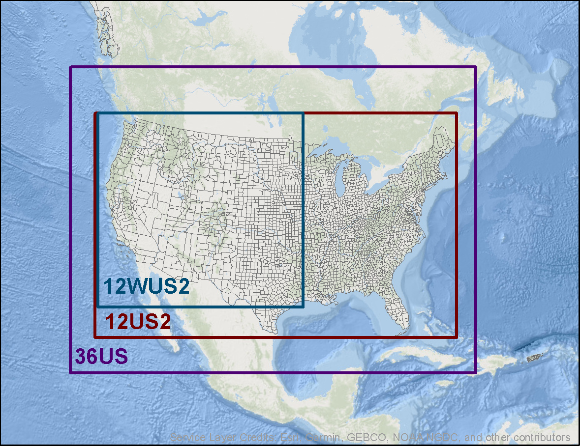
Figure 1. 36-km 36US, 12-km 12US2 and 12-km 12WUS2 modeling domains use in the 2014v1 Shake-Out PGM modeling.
The WAQS 12-km 12WUS2 and EPA 12-km 12US2 WRF output was
evaluated against observed surface wind speed, wind direction, temperature and
humidity (water mixing ratio) at surface monitoring sites in the western U.S.
The WAQS and EPA WRF precipitation were evaluated against monthly and daily PRISM
spatial maps in the western U.S. This resulted in 10s of thousands of WRF
model evaluation graphical displays. The WAQS and EPA comparative model
performance evaluation is summarized in Chapter 3 of the 2014v1
Shake-Out Draft Final Report and in a PDF
that was presented to the RTOWG on a January 31, 2019 webinar. All WRF MPE
graphical displays are available for viewing and download on the IWDW
Website where the user can drill down and analyze the 2014 WRF MPE to
individual states or even individual sites. There are three types of WAQS and
EPA 2014 MPE products available: (1) soccer plots that display surface
meteorological variability statistical performance measures against performance
goals and criteria across all western states, within each western states and at
individual monitoring sites; (2) time series plots of surface meteorological
variable model performance; and (3) comparison of observed and predicted
spatial plots of precipitation fields in the western U.S. by month and by
individual day. Figures 2 and 3 displays example soccer and time series plots
for the two 2014 WRF simulations and wind speed across the western U.S. An
example of WRF performance against PRISM data for August monthly precipitation
is shown in Figure 4.
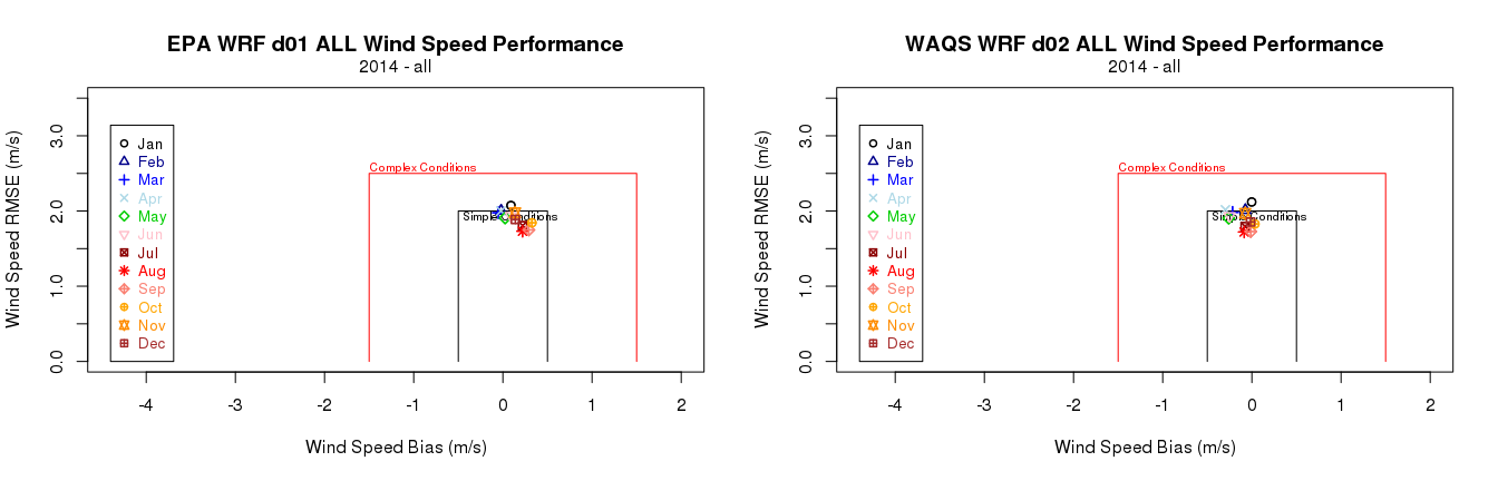
Figure 2. Example wind speed performance across western states for EPA (left) and WAQS (right) 2014 12-km WRF simulations.
Figure 3. Time series of daily predicted and observed wind speeds and wind speed bias (m/s) averaged across all sites in western U.S. for WAQS (blue) and EPA (red) WRF simulations and 2014 Q2 (left) and Q3 (right).
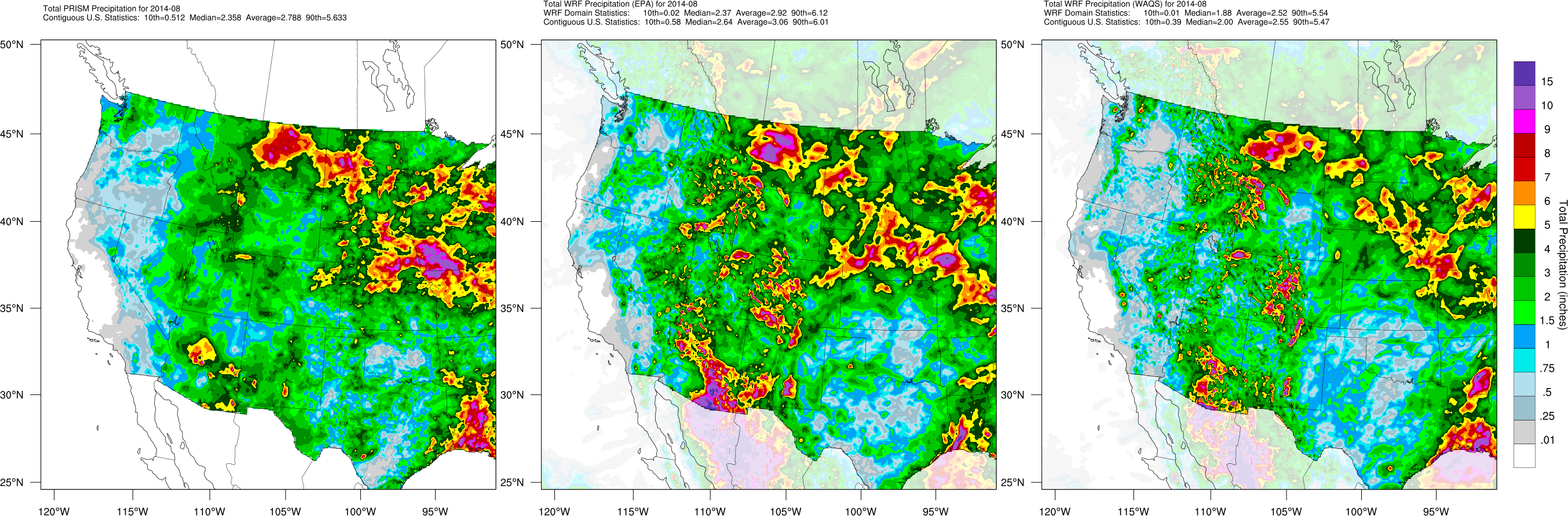
Figure 4. Comparison of August monthly total precipitation from PRISM (left) based on observations, EPA WRF (middle) and WAQS WRF (right).
The performance of the two 2014 WRF 12-km simulations varied
with no one WRF simulation exhibiting better performance across all
meteorological variables and locations than the other. For example, EPA WRF
produced better temperature performance, whereas WAQS WRF produced better wind
speed and summer precipitation performance. PGM sensitivity modeling of the
two 12-km WRF inputs that are presented in Chapter 5 of the 2014v1 Shake-Out
Draft Final Report found that one set of WRF fields did not produce better air
quality performance than the other across all species and locations.
Ultimately the WAQS 12-km 12WUS2 domain meteorological fields were selected for
the final 2014v1 Shake-Out CMAQ and CAMx simulations based on better summer
precipitation performance than the EPA 12-km WRF simulation.
2014v1 Base Case Emissions
The WRAP Shake-Out 2014v1 Base Case emissions are based on Version
2 of the 2014 National Emissions Inventory (2014NEIv2) with updates
provided by the WRAP western states. The CMAQ-ready 2014 emissions
inputs for 2014 and the 12-km 12US2 domain from the EPA 2014 Modeling Platform
were used for all source sectors but Point and Non-Point that had western
state updates so had to be re-processed. Details on the development of EPA’s
2014 modeling platform emissions are contained in their Technical Support
Document (TSD).
The SMOKE emissions model was used to process the 2014NEIv2 emissions with western
state updates to generate the 2014 12-km 12US2 domain CMAQ-ready emissions.
The 2014NEIv2 Mexico, Canada and off-shore shipping and oil and gas emission
sources were processed for the 36-km 36US domain. The CMAQ 2014 12-km 12US2
domain emissions were disaggregated to 36-km resolution and used to replace the
emissions in the 36-km 36US domain to make CMAQ-ready emissions for 2014 and
the 36-km 36US domain. The 2014v1 CMAQ-ready emissions were converted to the
CAMx format using the CMAQ2CAMx tool.
The WRAP Fire and Smoke Work Group made updates (e.g., classify
fires as either wildfire, prescribed burns and agricultural burning) to the
2014NEIv1 open land burning emissions that were then processed for input into
CMAQ and CAMx. The CAMx windblown dust (WBD) processor was used to generate
WBD emissions for both CMAQ and CAMx. The CAMx oceanic emissions processor was
used to generate sea salt (SSA) and dimethyl sulfide (DMS) emissions that were
used in CAMx. For CMAQ, the in-line SSA algorithm was used that does not
include DMS emissions. Note that because the version of CAMx (v6.5) used in
the 2014v1 Shake-Out modeling does not include explicit DMS chemistry, DMS was
renamed to SO2 when input into CAMx.
Chapter 2 of the 2014v1
Shake-Out Draft Final Report details the 2014v1 emissions data and
modeling with a summary contained in a PDF
that was presented at the April 5, 2019 2014v1 Shake-Out Close-Out meeting.
2014v1 Boundary Conditions
Boundary Condition (BC) concentrations for the most outer
36-km 36US PGM domain were defined using output from a 2014 GEOS-Chem global
chemistry model simulation EPA performed to define BCs for their CMAQ modeling
used in the 2014 National Air Toxics Assessment (NATA). EPA
used version 11-01 of GEOS-Chem with a horizontal resolution of 4 x 5 degrees
(~440 km) and 47 vertical levels. More details on EPA’s 2014 GEOS-Chem simulation
can be found in the 2014
NATA TSD. The output from EPA’s 2014 GEOS-Chem simulation were
processed to obtain BC inputs for CMAQ and CAMx and the 36-km 36US domain.
CAMx no emissions, inert chemistry and with deposition BC-only 2014 36/12-km
simulations were conducted and compared with observed concentrations. Since
there were no emissions, the CAMx BC-only simulations were expected to
under-predict the observed concentrations, however two overestimation problems
were revealed: (1) an ozone overestimation bias that occurs year-round; and (2)
a sulfate and SO2 overestimation bias during June and July. Additional CAMx
BC-only sensitivity simulations were performed with the 2014 GEOS-Chem BC
concentrations capped for some species as follows: ozone = 0.500 ppm (500 ppb);
sulfate = 2 µg/m3; and SO2 = 6 ppb. The ozone cap only affected
stratospheric ozone BC concentrations and the sulfate/SO2 caps only affected a
portion of the western BCs at the end of June and in early July. The cap on
the ozone BCs had little effect on the ozone overestimation bias that was due
to 2014 GEOS-Chem overstating tropospheric ozone concentrations. The cap on sulfate/SO2
BC concentrations alleviated with worst June/July SO4 overestimation bias.
Discussions with EPA revealed that they were aware of the
2014 GEOS-Chem ozone and sulfate performance issues and since it has minimal
effect on air toxics concentrations they did not try to correct them for their
2014 NATA modeling platform. The June/July sulfate/SO2 overestimation bias was
caused by using volcano eruption emissions in the 2014 GEOS-Chem run that uses
climatological volcano eruption emissions data that included a large eruption
in 2009 that was responsible for the sulfate/SO2 overestimation. EPA re-ran
their 2014 GEOS-Chem set-up turning off volcano eruption emissions whose
results were used for the June/July BCs in the final 2014v1 Shake-Out PGM simulations.
Details on the use of the 2014 GEOS-Chem BCs and sensitivity modeling are
contained in Chapter 4 of the 2014v1
Shake-Out Draft Final Report.
2014 PGM Sensitivity Tests
A limited amount of PGM sensitivity modeling was conducted
to investigate ways to improve model performance and identify model inputs and
model options for the final 2014v1 Shake-Out annual CMAQ and CAMx annual
simulations. The three main inputs examined in the sensitivity modeling were
BCs, meteorology and biogenic emissions that are documented in Chapters 4, 5
and 6, respectively, of the 2014v1 Shake-Out Draft Final Report and summarized
in the PDF file that was presented at the April 5, 2019 2014v1 Shake-Out Study
Close-Out meeting. Results of the comparison of the CAMx January and July 2014
BC, meteorological and biogenic emissions sensitivity tests with observations
are available in an Excel spreadsheet:
As discussed above, the PGM BC sensitivity modeling
identified that the 2014 GEOS-Chem BCs overstated ozone year-round and SO4/SO2
in the summer. The SO4/SO2 overstatement was corrected by having EPA rerun
GEOS-Chem for June and July 2014 without volcano emissions. Figure 5 displays
predicted and observed time series sulfate concentration at Yellowstone and
Weiminuche IMPROVE sites for the CAMx July 2014 BC sensitivity tests using 2014
GEOS-Chem BCs with and without volcano eruption emissions that clearly shows
the improved sulfate performance when volcano eruption emissions are not
included.
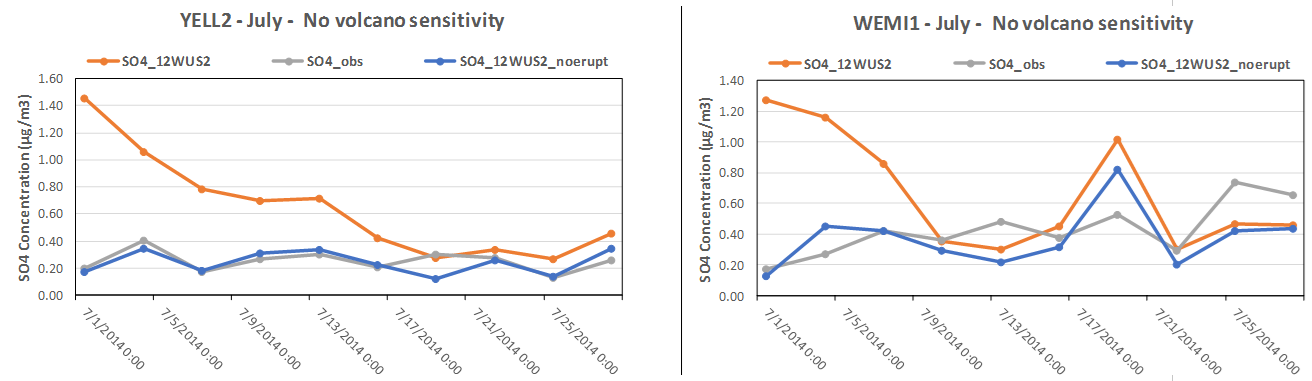
Figure 5. Predicted and observed sulfate concentrations at Yellowstone (left) and Weiminuche (right) IMPROVE sites for the CAMx July BC sensitivity tests using 2014 GEOS-Chem results with (orange) and without (blue) volcano eruption emissions.
The PGM meteorological sensitivity modeling ran CAMx for
January and July using the WAQS and EPA 12-km WRF meteorological inputs and
compared the CAMx model estimates with observations in a model performance
evaluation. Neither CAMx simulation using the two WRF meteorological inputs
exhibited consistently better model performance than the other (see Chapter 5
of 2014v1 Shake-Out Draft Final Report). For ozone, the comparison of model
performance was confounded by the overstated 2014 GEOS-Chem BCs. Ultimately
the WAQS 12-km WRF meteorological inputs were selected for the final 2014v1
Shake-Out PGM simulations based on better WRF summer precipitation model
performance.
Biogenic emissions sensitivity modeling conducted two CAMx
simulations of the 12-km 12WUS2 domain for January and July 2014, one using the
BEIS and the other using MEGAN3 biogenic emissions. The BEIS biogenic isoprene
emissions in the western U.S. tended to be approximately 20% lower than MEGAN3.
However, the BEIS terpene emissions were 4-5 times greater than MEGAN3. There
was a small effect of the biogenic emissions on ozone model performance but whether
one biogenic emissions model produced better ozone performance was difficult to
interpret due to the overstated ozone BCs. The different biogenic emission
models had a bigger effect on summer Organic Aerosol (OA) performance due to
the large differences in the biogenic terpene emissions that is a precursor to
Secondary Organic Aerosol (SOA). At most IMPROVE sites, the July 2014 CAMx OA
model performance was better using the BEIS biogenic emissions than MEGAN3 due
to higher OA concentrations that better matched the observed values. Figure 6
shows example OA time series plots at four IMPROVE sites in the western U.S.
with CAMx clearly showing better OA performance at the sites in CA (SEQU), WA
(NOCA) and CO (WEIM) but worse OA performance at the NM site (SAGU). Based on
the better summer OA model performance at most sites, the BEIS biogenic
emissions were selected for the final 2014v1 Shake-Out CMAQ and CAMx annual
simulations.
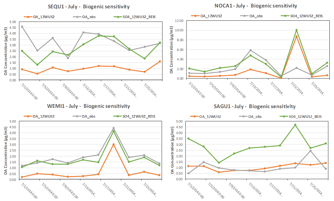
Figure 6. Predicted and observed time series of Organic Aerosol concentrations in July 2014 at the Sequoia CA, North Cascades WA, Weiminuche CO and Saguaro NM IMPROVE sites for the CAMx BEIS (green) and MEGAN (orange) biogenic emission sensitivity tests.
Final 2014v1 Shake-Out CMAQ and CAMx Simulations and Model Performance Evaluation
The final configuration for the 2014v1 Shake-Out annual CMAQ
and CAMx simulations used the revised 2014 GEOS-Chem simulation without volcano
eruption emissions for June and July to define BCs for the 36-km 36US. The
meteorological inputs for the 36/12-km domains were based on the WAQS 2014 WRF
simulation. BEIS biogenic emissions and the 2014v1 emissions with western
state updates were used. The table below summarizes the CMAQ and CAMx
configuration used in the final annual 2014v1 Shake-Out simulations and MPE.
| Science Options |
CAMx |
CMAQ |
Comment |
| Model Codes |
CAMx V6.5 - Apr 2018 |
CMAQ v5.2.1 – Apr 2018 |
CMAQ v5.3 Beta is available but will not be used as it needs more testing. |
| Horizontal Grid Mesh |
| 36 km grid |
148 x 112 cells |
148 x 112 cells |
36-km RPO CONUS |
| 12 km grid |
225 x 213 cells |
225 x 213 cells |
12-km WESTUS (12WUS2) WAQS |
| Vertical Grid Mesh |
25 vertical layers, defined by WAQS WRF |
25 vertical layers, defined by WAQS WRF |
Layer 1 thickness 20/24 m. Model top at ~19 km AGL |
| Grid Interaction |
One-way grid nesting |
One-way grid nesting |
CAMx and CMAQ 12-km 12WUS2 domain BCs based on 36-km CONUS CAMx and CMAQ simulations |
| Initial Conditions |
10 day spin-up on 36/12-km domains before January 1, 2014 |
10 day spin-up on 36/12-km domains before January 1, 2014 |
|
| Boundary Conditions |
Updated 2014 GEOS-Chem for 36-km CONUS domain |
Updated 2014 GEOS-Chem for 36-km CONUS domain |
EPA re-ran June and July 2014 GEOS-Chem without volcano eruptions |
| Emissions |
| Baseline Processing |
SMOKE, BEIS, CAMx Natural Emissions Processors |
SMOKE, BEIS, CMAQ in-line SSA and LNOx processors (CAMx WBD) |
2014NEIv2 with western state updates for Point and Non-Point |
| Sub-grid-scale Plumes |
Plume-in-Grid for major NOX sources (~300 in WUS) |
No Plume-in-Grid |
CMAQ does not have a Plume-in-Grid module |
| Chemistry |
| Gas Phase Chemistry |
CB6r4 |
CB6r3 |
Latest chemical reactions and kinetic rates with halogen chemistry (Yarwood et al., 2010) |
| Meteorological Processor |
WRFCAMx |
MCIP |
Compatible with CAMx v6.5 and CMAQ V5.2.1 |
| Horizontal Diffusion |
Spatially varying |
Spatially varying |
K-theory with Kh grid size dependence |
| Vertical Diffusion |
CMAQ-like Kv |
MCIP |
Minimum Kv 0.1 to 1.0 m2/s |
| Diffusivity Lower Limit |
Kz-min = 0.1 to 1.0 m2/s or 2.0 m2/s |
Kz-min = 0.1 to 1.0 m2/s or 2.0 m2/s |
Depends on urban land use fraction |
| Deposition Schemes |
|
|
|
| Dry Deposition |
Zhang dry deposition scheme |
CMAQ formulation |
(Zhang et. al, 2001; 2003) |
| Wet Deposition |
CAMx -specific formulation |
CMAQ formulation |
rain/snow/graupel |
| Numerics |
|
|
|
| Gas Phase Chemistry Solver |
Euler Backward Iterative (EBI) |
EBI |
EBI fast and accurate solver |
| Vertical Advection Scheme |
Implicit scheme w/ vertical velocity update |
CMAQ |
Emery et al., (2009a,b; 2011) |
| Horizontal Advection Scheme |
Piecewise Parabolic Method (PPM) scheme |
PPM |
Colella and Woodward (1984) |
| Integration Time Step |
Wind speed dependent |
Wind speed dependent |
1-5 min (12-km), 5-15 min (36-km) |
The 2014v1 Shake-Out CMAQ and CAMx annual 36/12-km
simulations were subjected to a multi-phased MPE. The Atmospheric Model
Evaluation Tool (AMET)
was used to evaluate the CMAQ and CAMx 2014v1 12-km modeling results using
observed gaseous and particle concentration data from the AQS, CSN, CASTNet and
IMPROVE monitoring networks. The IMPROVE observed particulate matter species
concentration data were then loaded into a spreadsheet to generate
visualization of the concentration data for the Most Impaired Days (MID) and
Worst 20% days and then processed into light extinction in a second spreadsheet
to analyze seasonal and daily performance. The Chapter 8 of the 2014v1
Shake-Out Draft Final Report discussed the CMAQ and CAMx 2014v1 MPE, with the
full suite of MPE products available in the links below.
AMET MPE Evaluation Products
AMET was run to generate scatter plots and spatial maps of
model performance statistics. The scatter plots included model performance statistics
and were generated for the annual period, by season and by month. The spatial
maps of model performance statistics were for the annual period. The species
considered in the AMET MPE analysis were gaseous Maximum Daily Average 8-hour
(MDA8) ozone concentrations and particle total PM2.5, SO4, NO3, NH4,
EC, OA, Na and Cl. All of the AMET graphical evaluation products can be viewed
using the Image Viewer below.
Figure 7 and 8 show example AMET MPE products for the 2914v1
CMAQ and CAMx simulation and DMA8 ozone and SO4 concentrations, respectively.
The DMA8 ozone scatter plots (Figure 7, top) are for all CASTNet sites in the
western U.S. and show a net overestimation bias (NMB) that is greater for CAMx
(+19%) than CMAQ (+11%). The spatial NMB bias plot for DMA8 ozone (Figure 7,
bottom) are all grey (≤±15%) or yellow and warmer colors with no cooler
(green-blue) colors indicating an ozone overestimations bias.
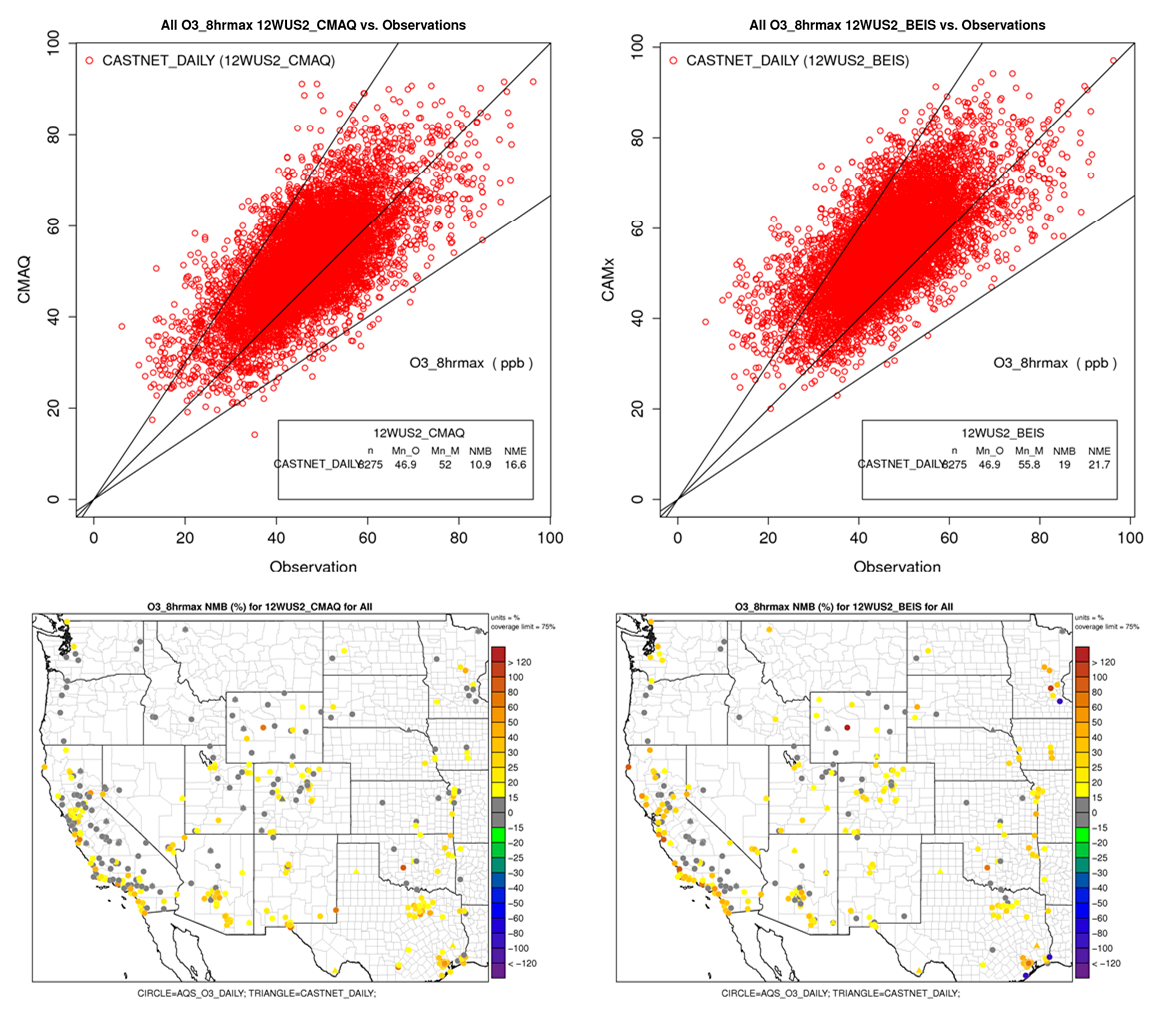
Figure 7. Example AMET MPE products for MDA8 ozone (O3_8hrmax) and CMAQ (left) and CAMx (right) 2014v1 Shake-Out runs showing scatter plots of CASTNet ozone (top) and Normalized Mean Bias (NMB) (bottom) across the 2014 annual period.
Both CMAQ and CAMx show fairly good SO4 performance across
the western U.S. for the 2014v1 base case simulations. CAMx has a few large
overpredictions that are mainly due to overstated SO4 at coastal sites (see NMB
bias plot in Figure 8, bottom right). This 2014v1 CAMx coastal summer SO4
overestimation will be investigated in the next phase of the study.
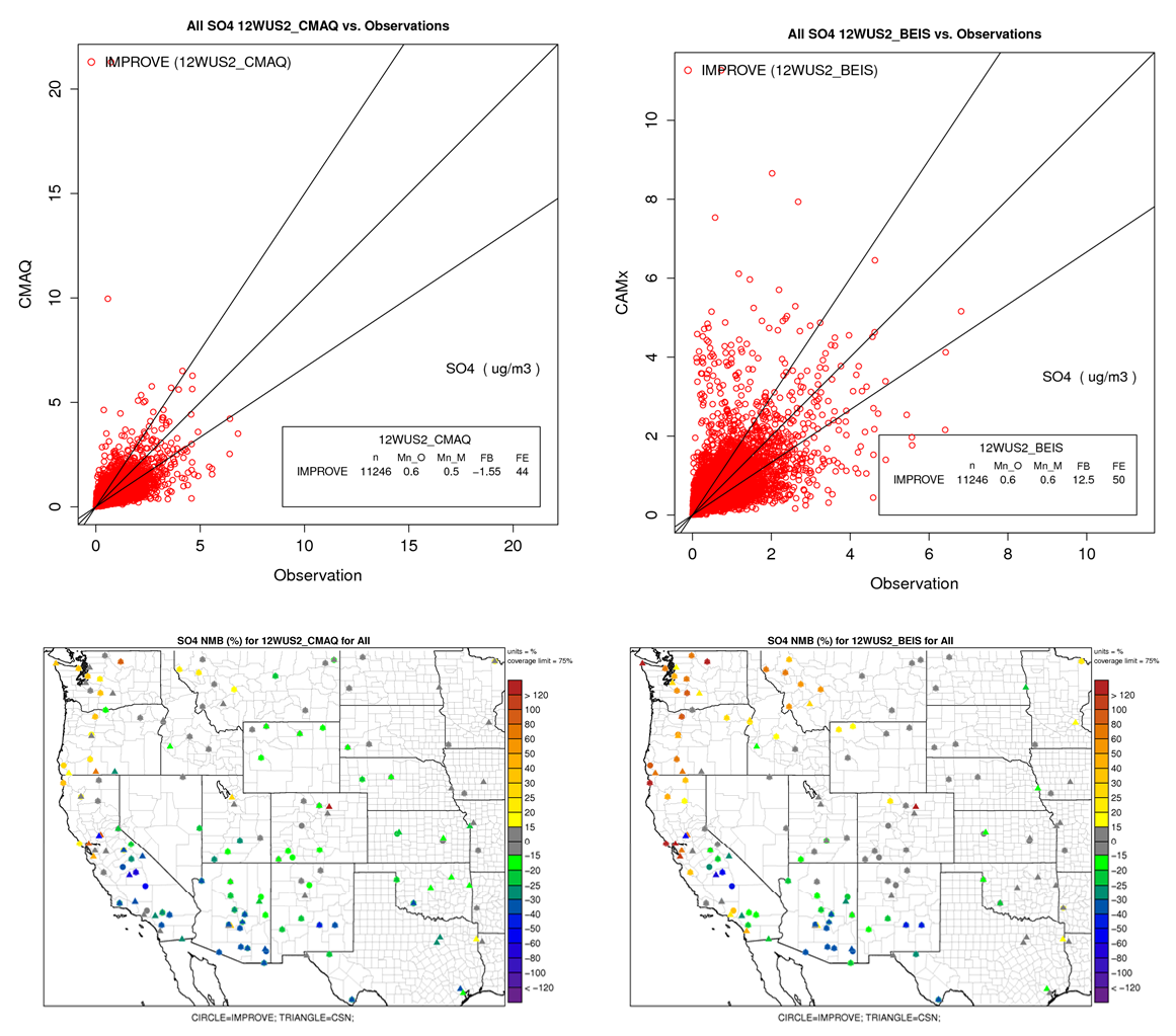
Figure 8. Example AMET MPE products for SO4 and CMAQ (left) and CAMx (right) 2014v1 Shake-Out runs showing scatter plots of IMPROVE SO4 (top) and Normalized Mean Bias (NMB) (bottom) across the 2014 annual period.
Time Series Evaluation Spreadsheet Tool
The AMET predicted and observed PM species concentration
pairs from the IMPROVE network were loaded into an Excel spreadsheet so that
time series comparisons could be made that the user could manipulate the time
period and concentration scale that is not possible with the AMET static time
series graphics. For example, when an IMPROVE site is impacted by concentrations
from file the automatic scaling is set to capture the high fire impact
conditions rendering the time series comparisons for the rest of the time difficult
to interpret. For example, Figure 9 shows time series of OA concentrations at
the Grand Canyon IMPROVE site using the auto-scaling approach and then with the
user setting the scale to a lower value so the comparisons can be seen for the
other days. The time series evaluation spreadsheet for the 2014v1 Shake-Out
CMAQ and CAMx simulations is available at the following link.
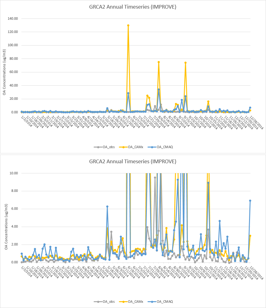
Figure 9. Time series of predicted and observed 24-hour average OA concentrations at Grand Canyon IMPROVE site for 2014v1 Shake-Out CMAQ (blue) and CAMx (orange) annual simulations using autoscaling (top) and user-defined scaling (bottom).
MID/W20% Days Concentration Evaluation Spreadsheet
The AMET predicted and observed PM species concentrations
from the IMPROVE network were loaded into an Excel spreadsheet and sorted by
the observed Most Impaired Days (MID) and Worst 20 percent (W20%) days so
comparisons could be made. These were some of the data that were used in the PDF
file that presented the 2014v1 Shake-Out CMAQ and CAMx MPE at the April 5, 2019
Close-Out meeting. Figure 10 shows example concentrations at Yellowstone
averaged across and for each individual observed MID and W20% days that shows
how the new MID visibility metric eliminates many observed days with high
wildfire contributions that are included in the W20% days (e.g., July 19). The
MID-W20% interactive spreadsheet of concentrations can be found at the
following link.
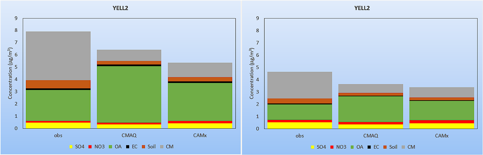
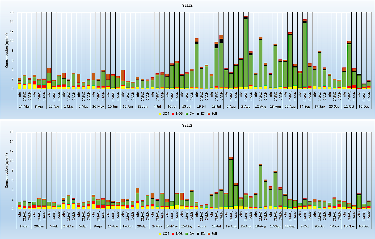
Figure 10. Predicted and observed PM concentrations at Yellowstone IMPROVE site average across the observed W20% (top left) and MID (top right) days and for each individual W20% (middle) and MID (bottom) days.
Light Extinction Evaluation Spreadsheet
The predicted and observed PM concentrations at the IMPROVE
sites were processed using the revised IMPROVE light extinction equation so
that the model performance for total PM extinction and extinction due to
individual components could be evaluated. The 2014v1 CMAQ and CAMx MPE for
light extinction is discussed in Chapter 8 of the 2014v1
Shake-Out Draft Final Report. The interactive spreadsheet of light
extinction (Mm-1) model performance can generate stacked bar charts
of total light extinction (without Rayleigh) and scatter and time series plots
of light extinction due to each PM component. Example displays of model
performance for the Mount Zirkel, Colorado IMPROVE site from the light
extinction MPE spreadsheet are shown in Figures 11 through 13 with the
spreadsheet available at the following link.
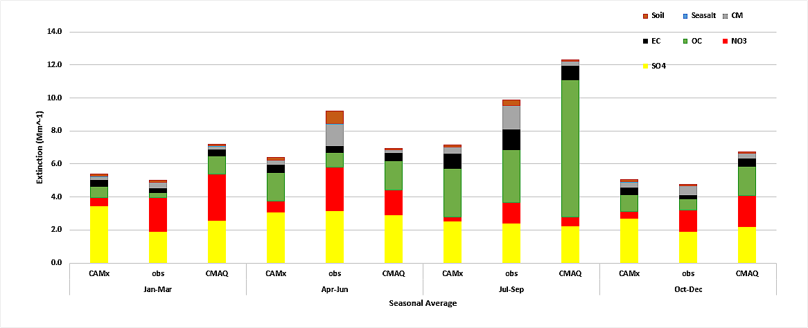
Figure 11. Predicted and observed stacked bar charts of seasonal light extinction (Mm-1) at Mount Zirkel IMPROVE site for the 2014v1 CMAQ and CAMx annual simulations.
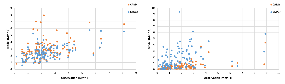
Figure 12. Scatter plot of predicted and observed daily ammonium sulfate (left) and ammonium nitrate (right) light extinction (Mm-1) at Mount Zirkel IMPROVE site for the 2014v1 CMAQ and CAMx annual simulations.
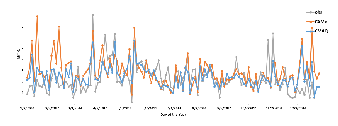
Figure 13. Time series plot of predicted and observed daily ammonium sulfate light extinction (Mm-1) at Mount Zirkel IMPROVE site for the 2014v1 CMAQ and CAMx annual simulations.
Major Model Performance Issues and Potential Resolution
The major model performance issues of the 2014v1 Shake-Out
CMAQ and CAMx annual simulations and recommendations for improvements are
presented in Chapter 9 of the 2014v1 Shake-Out Draft Final Report. They are
summarized as follows:
- Ozone: The ozone performance is dominated by the overstated BCs from EPA’s 2014 GEOS-Chem simulation. Rerunning GEOS-Chem using updated emissions and version of the model may alleviate this issue. Ozone in fire plumes frequently appears to be too high and the NOx speciation of fire emissions should be investigated and updated as needed.
- Sulfate: Once the problems with the June and July SO4/SO2 concentrations along the western BC was resolved by re-running GEOS-Chem without volcano eruptions, the SO4 performance was generally good with the exception of overstated SO4 at coastal sites by CAMx. Targeted sensitivity tests need to be performed using CAMx to identify the cause of this coastal SO4 overestimation bias so that corrective action can be taken. Because CAMx used different primary SO4 emissions from Sea Salt than CMAQ and included DMS emissions that were not in CMAQ, those are the first two variables to investigate in the CAMx coastal SO4 overestimation sensitivity tests.
- Nitrate: NO3 tends to be underestimated, with the underestimation greater in CAMx than CMAQ. The use of a bi-directional ammonia flux algorithm should be investigated along with the treatment of mineral (e.g., Ca and Na) nitrate.
- Organic Aerosol: In the absence of OA from fires, summer OA is overstated in the desert southwest that is believed to overstated SOA from biogenic terpene emissions. The treatment of biogenic emissions using BEIS and MEGAN should be re-visited.
- Elemental Carbon: EC performance is generally fairly good, although very uncertain when fire impacts occur.
- Other PM2.5/Soil: There and model-observed incommensurability issues with the Soil species that make them difficult to compare. The modeling of fine crustal species is challenging and can have local contribution that a grid model has difficulty simulating.
- Coarse Mass: Due to higher deposition rates, Coarse Mass (CM) is frequently dominated by local sources (e.g., road dust) that is subgrid-scale to the model so not well simulated and frequently underestimated.