WRAP/WAQS 2014v2 Modeling Platform Description and Western Region Performance Evaluation (MPE)
The CAMx 2014v2 36/12-km annual simulation was the final base case simulation used in the Western Regional Air Partnership (WRAP) Western Air Quality Study (WAQS) modeling.Figure 1 displays the 36-km continental U.S. (36US1) and 12-km western U.S. (12WUS2) modeling domains used in the WRAP/WAQS CAMx modeling.The meteorological inputs were based on the WAQS 2014 36/12/4-km WRF simulation and emissions were based on the 2014NEIv2 with western state updates.The CAMx 2014v2 base case modeling was built off
the CAMx 2014v1 Shakeout Study that developed the basic framework for the WRAP/WAQS 2014 modeling platform, conducted sensitivity modeling and recommended the configuration for the final CAMx 2014v2 base case simulation.The WRAP/WAQS 2014v1 Shakeout Study webpage contains details on the WRAP/WAQS 2014 platform development including the Final Modeling Plan, 2014v1 Shakeout Study Final Report, WAQS 2014 36/12/4-km WRF modeling used as
meteorological inputs for 2014v2, CAMx and CMAQ sensitivity modeling and 2014v1 MPE.
NOTE: This webpage contains information on the additional sensitivity tests conducted between the 20114v1 Shakeout and the final 2014v2 modeling and the model performance evaluation (MPE) of the final CAMx 2014v2 36/12-km base case simulation.
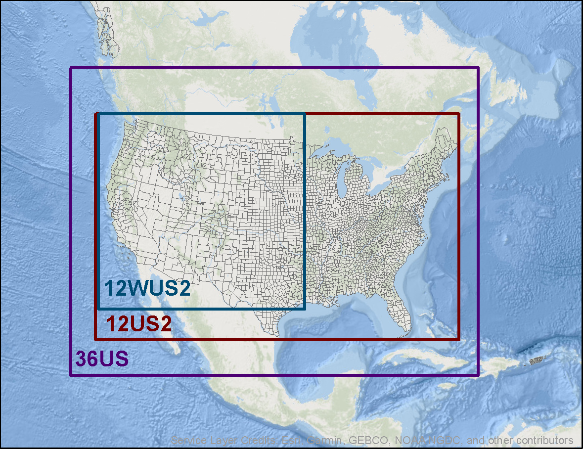
Figure 1. 36-km continental U.S. (36US1) and 12-km western U.S. (12US2) modeling domains used in the WRAP/WAQS CAMx 2014v2 base case simulation.
Sensitivity Modeling Leading to Final CAMx 2014v2 Configuration
The following were the major model performance issues in the preliminary CAMx and CMAQ 2014v1 Shakeout Study base case simulations, with details provided in Chapter 9 of the 2014v1 Shakeout Final Report:
- Ozone (O3): The ozone performance is dominated by a year-round large overestimation tendency, particularly in the colder months. The cause of the overestimation was traced to overstated ozone Boundary Conditions (BCs) from EPA’s 2014 GEOS-Chem simulation that defined the BCs in EPA’s 2014 modeling platform used in the 2014 National Air Toxics Assessment (NATA).
- Sulfate (SO4): Once problems with the June and July SO4/SO2 concentrations along the western BC was resolved by re-running EPA’s 2014 GEOS-Chem for June/July without volcano eruptions, the SO4 performance was generally reasonable with the exception of overstated SO4 in the Pacific North West (PNW) and at coastal sites.
- Nitrate (NO3): NO3 tended to be underestimated, with the underestimation greater in CAMx than CMAQ.
- Organic Aerosol (OA)/Organic Carbon (OC): In the absence of OA from fires, OA was reasonable given the uncertainties, except summer OA is overstated in the desert southwest.
- Elemental Carbon (EC): EC performance is generally fairly good, although very uncertain when fire impacts occur.
- Other PM2.5/Soil: There are model-observed incommensurability issues with the Soil species that make them difficult to compare (e.g., IMPROVE Soil based on linear combination of Elements and CAMx other PM2.5 remaining PM2.5 not explicitly speciated). The modeling of fine crustal species is challenging and can have local contribution that a grid model has difficulty simulating.
- Coarse Mass (CM): Due to higher deposition rates and settling velocities, Coarse Mass (CM) is frequently dominated by local sources (e.g., road dust) that is subgrid-scale to the model so not well simulated. CM is underestimated when large natural dust storms occur that are not reproduced by the models.
Additional CAMx sensitivity tests were conducted, as described below, to try and improve the model performance over the 2014v1 Shakeout base case and define the optimal 2014v2 model configuration.
WRAP 2014 GEOS-Chem Modeling for New Boundary Conditions (BCs)
To address the year-round ozone large overestimation tendency in the initial 2014v1 base case simulations, WRAP performed a revised 2014 GEOS-Chem simulation using the latest emissions inventory information and a newer version of the model. The results of the WRAP revised 2014 GEOS-Chem simulation and CAMx sensitivity modeling using the new BCs were presented at the September 10, 2019 RTOWG Webinar. Figure 2 reproduces results from that Webinar and shows predicted and observed maximum daily average 8-hour (MDA8) ozone time series comparisons at Lassen Volcanic National Park in northern California and Yellowstone National Park, Wyoming using the EPA and WRAP 2014 GEOS-Chem BCs. In January, the CAMx simulation using the WRAP 2014 GEOS-Chem BCs is clearly performing much better than when the BCs based on EPA’s 2014 GEOS-Chem run are used with the large ozone overestimating bias eliminated. In July, the differences are not as great, but CAMx with the WRAP 2014 GEOS-Chem BCs is performing marginally better than using the EPA’s 2014 GEOS-Chem BCs.
Figure 2. Comparison of predicted and observed (black) MDA8 ozone concentrations (ppb) in January (left) and July (right) 2014 at Lassen Volcanic, California (top) and Yellowstone, Wyoming (bottom) CASTNet sites for CAMx using BCs based on the original EPA 2014 GEOS-Chem simulation (blue) and BCs based on the revised WRAP 2014 GEOS-Chem simulation (purple).
Coastal SO4 Overestimation
The CAMx 2014v1 simulation overstated the summer observed SO4 concentrations at coastal monitoring sites, such as Point Reyes (PORE) and Redwood (REDW) in California. Several CAMx zero-out emission sensitivity simulations were conducted to investigation the contribution of primary SO4 emissions in sea spray aerosol (SSA) and emissions of oceanic Dimethyl Sulfide (DMS), as well as using explicit DMS chemistry (the CAMx 2014v1 simulation renamed DMS as SO2 since the version of CAMx used did not include DMS chemistry). Eliminating SSA primary SO4 emissions had little effect on the predicted coastal SO4 concentrations. Eliminating DMS emissions reduced the coastal SO4 overestimation bias by approximately half. Explicit DMS chemistry had a small effect on coastal SO4 predictions. No changes were made in the modeling so the IMPROVE sites on the coast still have a summer SO4 overestimation bias in the final CAMx 2014v2 base case simulation. Details on the coastal SO4 CAMx sensitivity test are available in the presentation given at the September 10, 2019 RTOWG Webinar. Ultimately the contributions to summer coastal SO4 concentrations were assessed using CAMx source apportionment modeling and found the largest contributors were BCs due to international anthropogenic emissions, BCs due to natural sources and natural sources from within the CAMx modeling domain (mainly DMS).
Bi-Directional Ammonia Deposition
The latest version of CAMx includes a bi-directional (bidi) ammonia deposition scheme that allows deposited ammonia concentrations to be resuspended in the atmosphere. CAMx sensitivity tests were run with and without the CAMx bidi ammonia deposition scheme and found that use of the bidi ammonia module resulted in slightly higher NO3 concentrations and better winter NO3 model performance (see link for September 10, 2019 RTOWG Webinar given above for details). Given that CAMx underestimated the observed winter NO3 when NO3 is an important part of the visibility extinction, the bidi ammonia scheme was adopted for the final CAMx 2014v2 base case simulation.
Fire Plume Rise Sensitivity Modeling
The processing of the 2014 NEI fires with SMOKE uses the Briggs plume rise algorithm took several weeks to conduct, generated hundreds of thousands of virtual point sources for input into CAMx and used excessive amount of disk space. This resulted in a very computationally intensive set-up for both processing the fire emissions and running the CAMx simulations that had to input and store in memory 100,000s of fire point sources. The WRAP plume rise algorithm uses a plume top and bottom and CAMx internally determines the vertical layers fire emissions are injected so is more computationally efficient. Fire plume rise sensitivity modeling was conducted and presented at the November 19, 2019 RTOWG Webinar and found comparable performance using the two fire plume rise algorithms. Thus, the more computationally efficient WRAP plume rise approach was adopted for final CAMx 2014v2 base case.
Updated 2014v2 Emissions
Western states provided emission updates to 2014v1 emissions that were implemented in 2014v2 base case emissions scenario. The largest change was for California where the Air Resources Board (ARB) provided a complete replacement to the 2014v1 California emissions, which were based on the 2014NEIv2. The total emissions in the new California 2014v2 inventory were fairly similar to 2014v1, except for ammonia that had approximately half the emissions in 2014v2 compared to 2014v1. Details on the 2014v2 emission updates are given in the September 10, 2019 RTOWG Webinar referenced earlier.
CAMx Version 7 Sensitivity
A sensitivity test was conducted using the beta6 version of CAMx v7 that included explicit treatment of Elements so that the Soil species can be defined in a consistent fashion between the model and IMPROVE measurements. CAMx v7 has other improvements, including explicit DMS chemistry and the ability for source apportionment to track BC segment contributions that is proving valuable for estimating the contributions of international anthropogenic emissions. The current CAMx regional haze modeling is using the publicly available version of CAMx v7.0 that was released in May 2020 whose source code, user’s guide and other processors and information are available on the CAMx Website.
Final CAMx 2014v2 Model Configuration
Table 1 below lists the CAMx configurations for the 2014v1 Shake-Out and final 2014v2 base case simulations. The largest changes in the CAMx 2014v2 configuration were:
- CAMx v7.0.
- Updated BCs using new WRAP 2014 GEOS-Chem run.
- Updated 2014v2 emissions.
- Use of ammonia bi-directional deposition flux scheme.
- Explicit DMS chemistry.
- Mapping of CMAQ SOAALK species in the emissions to CAMx SOA precursor species.
Due to time and resource constraints, the CMAQ model was not carried forward to the 2014v2 platform. EPA released a new CMAQ v5.3 in August 2019 that has to use MCIPv5.0 meteorological inputs so the 2014 WRF data would have to be re-processed. In addition, MCIPv5.0 no longer supports layer collapsing resulting in CMAQ run times that are much longer (almost 2x) than CAMx.
Table 1. Comparison of CAMx model configuration between the 2014v1 preliminary and 2014v2 final base case simulations
| Science Options |
2014v1 |
2014v2 |
Comment |
| Model Codes |
CAMx V6.5 - Apr 2018 |
CMAQ v7 – May 2020 |
CAMx v7beta6 used for 2014v2 |
| Horizontal Grid Mesh |
| 36 km grid |
148 x 112 cells |
148 x 112 cells |
36-km RPO CONUS |
| 12 km grid |
225 x 213 cells |
225 x 213 cells |
12-km WESTUS (12WUS2) WAQS |
| Vertical Grid Mesh |
25 vertical layers, defined by WRF |
25 vertical layers, defined by WRF |
Layer 1 thickness 20/24 m. Model top at ~19 km AGL |
| Grid Interaction |
One-way grid nesting |
Two-way grid nesting |
|
| Initial Conditions |
10 day spin-up |
10 day spin-up |
Run in quarters |
| Boundary Conditions |
EPA 2014 GEOS-Chem |
WRAP 2014 GEOS-Chem |
WRAP re-ran 2014 GEOS-Chem to improve BCs |
| Emissions |
| Processing |
SMOKE, BEIS, CAMx Processors |
SMOKE, BEIS, CMAQ in-line processors |
2014NEIv2 with western state updates for Point and Non-Point |
| Sub-grid-scale Plumes |
Plume-in-Grid for major NOX sources |
Plume-in-Grid for major NOX sources |
|
| Chemistry |
| Gas Phase Chemistry |
CB6r4 |
CB6r6 |
Latest chemical reactions and kinetic rates with halogen chemistry (Yarwood et al., 2010) |
| Meteorological Processor |
WRFCAMx |
WRFCAMx |
|
| Horizontal Diffusion |
Spatially varying |
Spatially varying |
K-theory with Kh grid size dependence |
| Vertical Diffusion |
CMAQ-like Kv |
CMAQ-like Kv |
Minimum Kv 0.1 to 1.0 m2/s |
| Diffusivity Lower Limit |
Kz-min = 0.1 to 1.0 m2/s or 2.0 m2/s |
Kz-min = 0.1 to 1.0 m2/s or 2.0 m2/s |
Depends on urban land use fraction |
| Deposition Schemes |
|
|
|
| Dry Deposition |
Zhang dry deposition scheme |
Zhang dry deposition scheme |
(Zhang et. al, 2001; 2003) |
| Wet Deposition |
CAMx -specific formulation |
CAMx -specific formulation |
rain/snow/graupel |
| Numerics |
|
|
|
| Gas Phase Chemistry Solver |
Euler Backward Iterative (EBI) |
Euler Backward Iterative (EBI) |
EBI fast and accurate solver |
| Vertical Advection Scheme |
Implicit scheme w/ vertical velocity update |
Implicit scheme w/ vertical velocity update |
Emery et al., (2009a,b; 2011) |
| Horizontal Advection Scheme |
Piecewise Parabolic Method (PPM) scheme |
Piecewise Parabolic Method (PPM) scheme |
Colella and Woodward (1984) |
| Integration Time Step |
Wind speed dependent |
Wind speed dependent |
1-5 min (12-km), 5-15 min (36-km) |
CAMx 2014v2 Model Performance Evaluation
The CAMx 2014v2 36/12-km base case simulation was subjected to a model performance evaluation (MPE) for ozone and PM concentrations and visibility extinction based on PM concentrations. Version 1.4 of the Atmospheric Model Evaluation Tool (AMET) was the primary tool used to evaluate the CAMx 2014v2 base case simulation, although data was also ported to the WRAP Technical Support System (TSS) where MPE products comparing the observed and modeled visibility extinction on the Most Impaired Days (MID) and clearest days can be generated. The CAMx 2014v2 MPE provided below has the following elements:
- Comparison of the WRAP/WAQS CAMx 2014v2 MPE against EPA’s CAMx 2016beta’ base case that was used in EPA’s national 2028 regional haze modeling that was released in September 2019.
- Evaluation of the CAMx 2014v2 base case against visibility extinction for the 2014 IMPROVE MID and clearest days.
- Evaluation of CAMx 2014v2 base case for ozone and PM concentrations using a suite of AMET evaluation displays.
Statistical Model Performance Metrics and Model Performance Goals and Criteria
A standard set of statistical performance metrics were calculated by AMET as follows:
Mean bias (MB) is the average difference between predicted (P) and observed (O) concentrations for a given number of samples (n):
Mean error (ME) is the average absolute value of the difference between predicted and observed concentrations for a given number of samples:
Normalized mean bias (NMB) is the sum of the difference between predicted and observed values divided by the sum of the observed values:
Normalized mean error (NME) is the sum of the absolute value of the difference between predicted and observed values divided by the sum of the observed values:
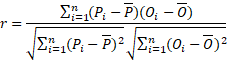
Pearson’s correlation coefficient (r) is defined as:
Model performance goals and criteria are used to aid in the evaluation of the model and put the model evaluation into context with past model performance evaluations. EPA’s 1991 ozone guidance presented the first ozone performance goals for bias (≤±15%) and error (≤±15%). However, EPA’s latest November 2018 guidance for ozone, PM2.5 and regional haze modeling does not endorse any specific model performance goals and criteria. Simon, Baker and Phillips (2012) summarized the model performance statistics from 69 PGM applications from 2006 to 2012 and found lots of variability, but were able to isolate model performance statistical levels for the best performing models. Emery et al., (2016) built off the work of Simon, Baker and Phillips (2012) adding additional PGM model applications and coming up with a set of PGM model performance goals and criteria based on the variability in past PGM model performance. “Goals” indicate statistical values that approximately a third of the top performing past PGM applications have met and should be viewed as the best a model can be expected to achieve. “Criteria” indicates statistics values that approximately two thirds of past PGM applications have met and should be viewed as what a majority of the models have achieved. The model performance goals and criteria are not only used to help judge model performance, but are also integral parts of some model performance displays, such as soccer plots. Table 2 lists the model performance goals and criteria by species that were adopted in the CAMx 2014v2 base case MPE.
Table 2. Recommended performance goals and criteria benchmarks for photochemical model statistics (Source: Emery et al., 2016)
| Species |
NMB |
NME |
r |
| Goal |
Criteria |
Goal |
Criteria |
Goal |
Criteria |
| 1-hr & MDA8 Ozone |
<±5% |
<±15% |
<15% |
<25% |
>0.75 |
>0.50 |
| 24-hr PM2.5, SO4, NH4 |
<±10% |
<±30% |
<35% |
<50% |
>0.70 |
>0.40 |
| 24-hr NO3 |
<±15% |
<±65% |
<65% |
<115% |
NA |
NA |
| 24-hr OC |
<±15% |
<±50% |
<45% |
<65% |
NA |
NA |
| 24-hr EC |
<±20% |
<±40% |
<55% |
<75% |
NA |
NA |
Comparison of WRAP/WAQS CAMx 2014v2 and EPA’s 2016beta’ Base Cases Model Performance Evaluation
On September 19, 2019, EPA released their updated 2028 national regional haze modeling using the CAMx model and the EPA 2016beta’ modeling platform. The MPE of the CAMx 2016beta’ base case is presented in Appendix A of the Technical Support Document (TSD) for EPA’s 2028 national regional haze modeling. EPA evaluated the CAMx 2016beta’ base case simulation by U.S. Climate Regions as shown in Figure 3.
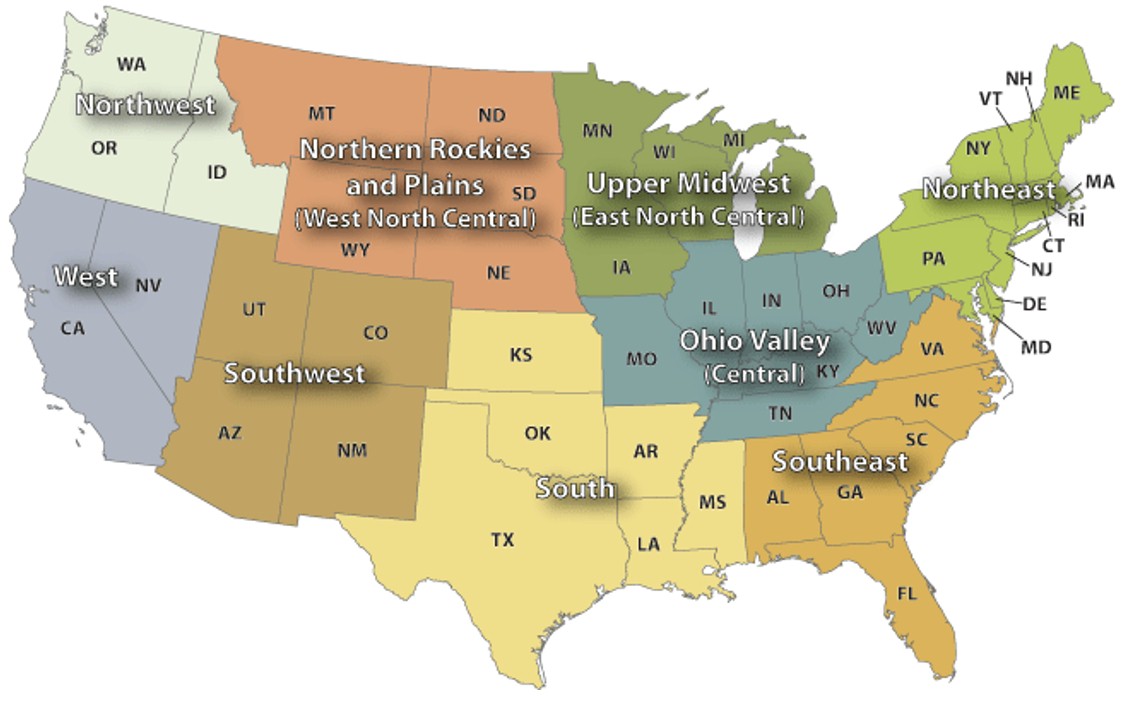
Figure 3. U.S. Climate Regions used to evaluate the EPA CAMx 2016beta’ base case simulation.
The WRAP/WAQS evaluation of the CAMx 2014v2 36/12-km base case simulation also adopted the U.S. Climate Regions that were fully or near fully contained within the 12-km 12WUS2 modeling domain. The WRAP/WAQS CAMx 2014v2 12-km model performance was compared against EPA’s
CAMx 2016beta’ 12-km model performance using two types of MPE products that were common from the WRAP/WAQS AMET MPE and the EPA MPE in their TSD:
- Spatial maps of site-specific Mean Normalized Bias (NMB) and Mean Normalized Error (NME) for PM species (e.g., SO4, NO3, OA, EC and Soil).
- Kellygrams that displays a matrix of NMB and NME of PM species by season and U.S. Climate Region.
Some manipulation of the EPA CAMx 2016beta’ evaluation displays had to be made to make them comparable for direct comparison with the CAMx 2014v2 AMET evaluation products. A PowerPoint presentation of side-by-side comparisons of the EPA 2015beta’ CAMx and WRAP/WAQS 2014v2 CAMx MPE products for the spatial maps of site-specific NMB and Kellygrams of NMB by season and U.S. Climate regions in the western states is provided in the link below:
Figures 4 and 5 show examples of the site-specific SO4 NMB performance for the WRAP/WAQS CAMx 2014v2 (left) and EPA CAMx 2016beta’ (right) base case simulations using the AMET spatial statistical metric output. The SO4 performance is mixed with the EPA CAMx 2016beta’ base case exhibiting a much larger Winter SO4 overestimation bias than 2014v2. But EPA’s 2016beta’ CAMx simulation performs better at inland IMPROVE sites in the WRAP states for summer SO4, although it has a larger SO4 overestimation bias in the Northwest Climate Region.
An example Kellygram for NO3 performance is shown in Figure 6. The WRAP 2014v2 CAMx run NO3 has an overestimation tendency, although it performs better in the winter than 2016beta’when NO3 is a larger and more important component of visibility extinction and PM2.5.
Figure 4. Example spatial maps of site-specific Winter SO4 Mean Normalized Bias (MNB) for the WRAP/WAQS 2014v2 (left) and EPA 2016beta’ (right) CAMx base case simulations.
Figure 5. Example spatial maps of site-specific Summer SO4 Mean Normalized Bias (MNB) for the WRAP/WAQS 2014v2 (left) and EPA 2016beta’ (right) CAMx base case simulations.
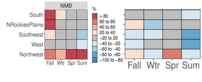
Figure 6. Example Kellygrams for NO3 Normalized Mean Bis (NMB) that display the WRAP/WAQS CAMx 2014v2 (left) and EPA 2016beta’ (right) CAMx base case performance by season and U.S. Climate Regions.
Evaluation of Visibility Extinction for the IMPROVE 2014 MID and Clearest Days
The first two products in the WRAP TSS Model Data Analysis – Express Tools provide a comparison of the observed and CAMx predicted extinction for the 2014 IMPROVE MID and clearest days. The first TSS modeling Express Tools product displays stacked bar charts of extinction at IMPROVE sites averaged across the 2014 IMPROVE MID and clearest days. There are three user-defined settings: (1) the state defining the IMPROVE sites for display; (2) MID or clearest days; and (3) 2014v2 or RepBase CAMx simulations. Figures 7 and 8 display the CAMx 2014v2 MPE averaged across the 2014 IMPROVE MID and clearest days at the Mount Zirkel (MOZI1) IMPROVE site in Colorado from the first TSS modeling Express Tool. Although the model tends to predict the observed total extinction averaged across the 2014 IMPROVE MID well (within 5%), it underestimates the SO4, overestimates the NO3 and OA and underestimations Soil and CM extinction at MOZI1. The model tends to overestimate the extinction on the 2014 observed clearest days at MOZI1 (Figure 8), which is a common occurrence across IMPROVE sites for the clearest days.
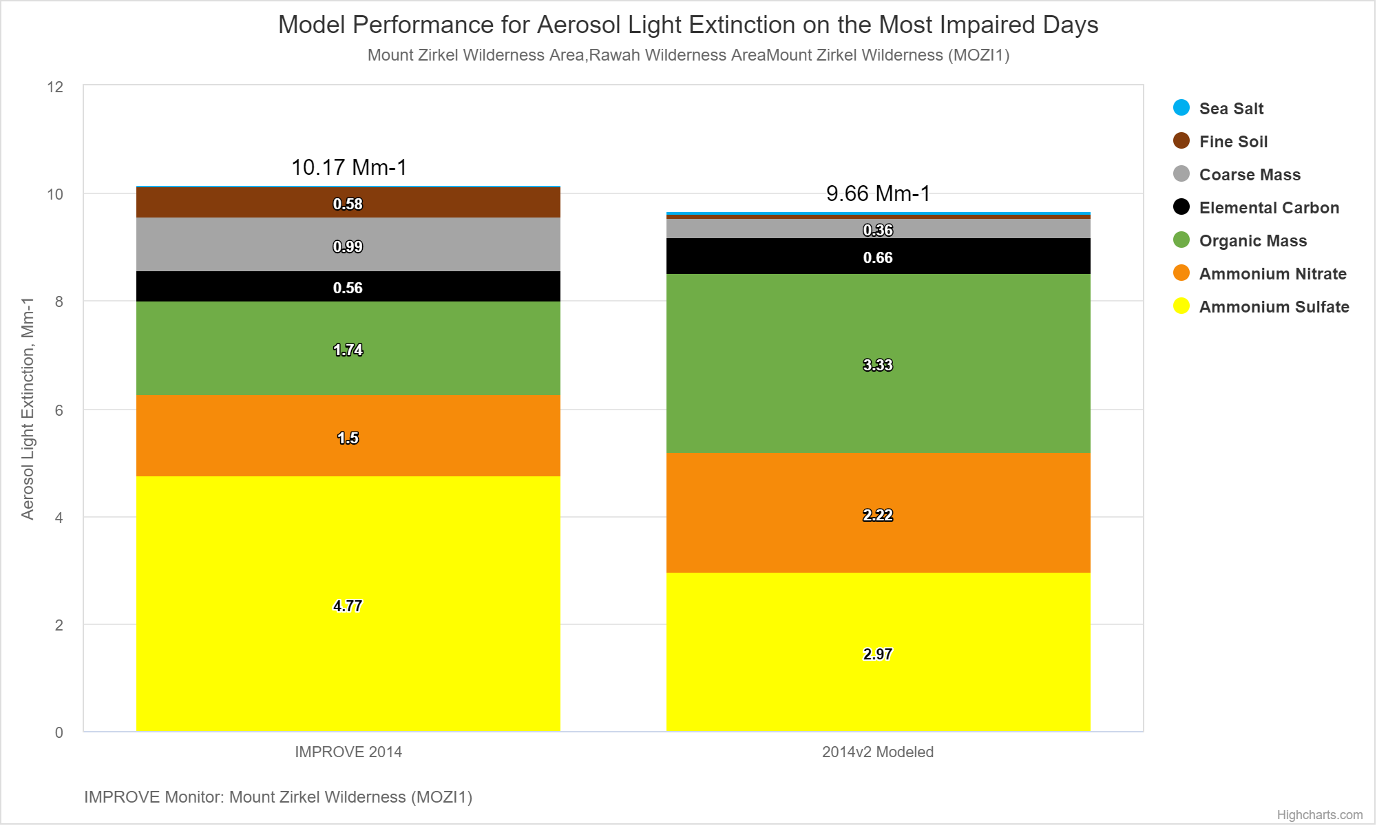
Figure 7. Observed (left) and CAMx 2014v2 predicted (right) visibility extinction at MOZI1 averaged across the IMPROVE 2014 MID.
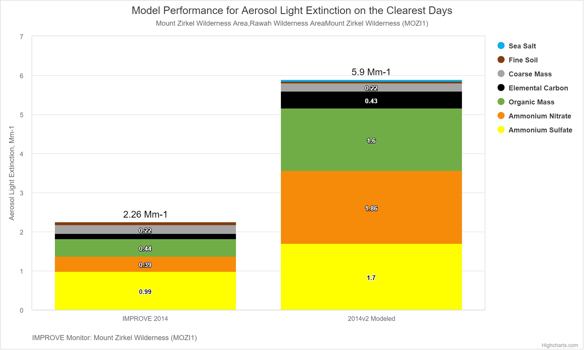
Figure 8. Observed (left) and CAMx 2014v2 predicted (right) visibility extinction at MOZI1 averaged across the IMPROVE 2014 20% clearest days.
The second product in the modeling Express Tools on the WRAP TSS website provides an evaluation for the IMPROVE 2014 MID and clearest days on a daily basis. Figure 9 shows an example of the daily MPE at MOZI1 for the 2014 IMPROVE MID. In this case displays for both the 2014v2 and RepBase CAMx emission scenarios were selected to compare against the observed daily extinction.
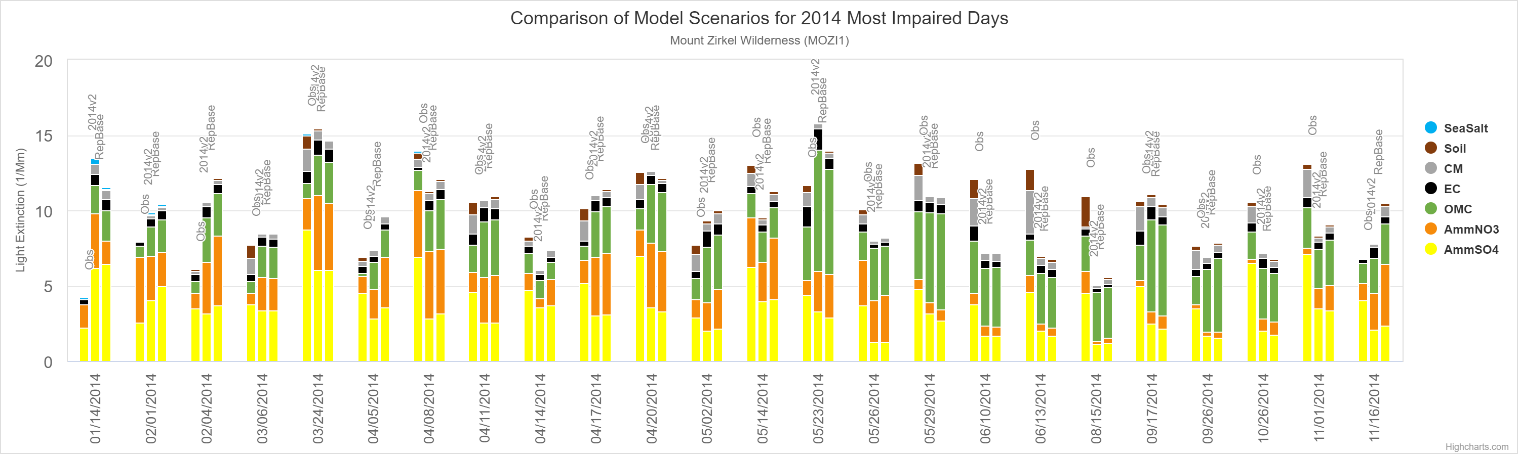
Figure 9. Comparison of the observed and 2014v2 and RepBase CAMx predicted daily visibility extinction on the 2014 IMPROVE MID at the MOZI1 IMPROVE site.
Comparisons of the CAMx 2014v2 model performance for visibility extinction are available from the TSS Express Tool with additional examples also provided for selected sites in each Climate Region in the PowerPoint/PDF document of example AMET displays given in the next section.
CAMx 2014v2 AMET MPE Products
EPA’s AMET v1.4 MPE tool was applied to evaluate the CAMx 2014v2 base case simulation concentrations. Numerous AMET MPE products were generated for the entire 12-km 12WUS2 domain and Climate Regions (Figure 2) that were contained or mostly contained within the western U.S. 12-km 12WUS2 modeling domain (Figure 1) as follows:
- Northwest
- West
- Northern Rockies and Plains
- Southwest
- South
AMET was applied to evaluate the CAMx 2014v2 base case simulation for concentrations within monitoring network sites within the 12-km 12WUS2 modeling domain as well as separately for sites within each of the five U.S. Climate Regions listed above. The species mapping between the modeled and measured species in the IMPROVE network are available in an IMPROVE-CAMx Species Mapping Excel Spreadsheet. The AMET species name and simple definition for the IMPROVE monitoring network species are shown in Table 3. Measured data from the CSN network were also included in some of the PM species evaluation products using similar species mappings as IMPROVE. The ozone evaluation was conducted for Maximum Daily Average 8-hour (MDA8) ozone concentrations (O3_8hrmax in AMET) from the CASTNet and AQS monitoring networks.
Table 3. Species from the IMPROVE monitoring network evaluated using AMET MPE products and their simple explanation.
| Species |
Simple Explanation |
| Cl |
Chlorine, primarily from sea salt |
| EC |
Elemental Carbon, also called Light Absorbing Carbon (LAC) or Black Absorbing Carbon (BAC) |
| Na |
Sodium, primarily from sea salt and dust |
| NH4 |
Ammonium, for IMPROVE network NH4 is derived from SO4 and NO3 assuming they are completely neutralized by NH4 |
| NO3 |
Nitrate |
| OC |
Organic Carbon, modeled OA species are converted to OC |
| Other |
Other PM2.5, includes Soil and other PM2.5 not SO4, NO3, NH4, OA and EC |
| PM10_2 |
Observed is PM10 mass measurement, modeled is sum of all modeled PM10 species |
| PM10 |
Observed is PM10 mass measurement, modeled uses IMPROVE SOIL liner combination of Elements and drops the FPRM, FCRS, CPRM and CCRS species |
| PM2.5_2 |
Observed is PM2.5 mass measurement, modeled is sum of all modeled PM2.5 species |
| PM2.5 |
Observed is PM2.5 mass measurement, modeled uses IMPROVE SOIL liner combination of Elements and drops the FPRM and FCRS species |
| PMC |
Coarse Mass (CM) |
| SO4 |
Sulfate |
| Soil |
2.20*Al+2.49*Si+1.63*Ca+2.42*Fe+1.94*Ti |
The AMET evaluation products are available from an Image Browser using the link given below. Over 10,000 graphical displays of MPE are available through the Image Browser. The directory structure for the Image Browser starts with the "2014v2" root folder that has two subfolders of "climate_regions" and "Fulldomain_12wus2" that indicate the geographic region for which the AMET MPE products were generated. The "Fulldomain_12wus2" folder has the following AMET MPE products:
MPE Displays in the "Fulldomain_12wus2" Folder
- "kellyplot": contains kellygrams that displays a matrix of model performance statistics for PM species and ozone by season (x-axis) and Climate Regions (y-axis), see examples in Figures 6 and 10. For common PM species in the IMPROVE and CSN networks, separate Kellygrams are generated to help differentiate model performance in these more rural-oriented and more urban-oriented monitoring networks, respectively.
- "scatter_plots": contains scatter plots of predicted and observed concentrations across all data in the 12WUS2 domain for the annual period and by season. Scatter plots are available for ozone across the CASTNet and AQS networks and for PM species across the IMPROVE network along or the combined IMPROVE and CASTNet networks.
- "soccer_plots": typically plot bias (x-axis) versus error (y-axis) and display boxes representing performance goals and criteria so it is easy to recognize when the bias and error performance metrics achieve them. We present soccer plots of monthly NMB vs. NME for the whole 12WUS2 domain using the performance goals and criteria in Table 2.
- "stats_plots": contain spatial maps of site-specific MPE performance metrics for the annual and seasonal periods and ozone and PM species. MPE performance metrics include bias (MB, NMB and FB), error (ME, NME, FE and RMSE) and correlation (Corr). For PM species, performance metrics for both IMPROVE and CSN sites are included in the spatial maps.
- "timeseries": contain site-specific time series of predicted and observed concentrations at CASTNet (DMAX8 ozone) and IMPROVE (PM species) sites within the 12WUS2 domain.
The "climate_regions" folder contains a "scatter_plots" and "soccer_plots" subfolders that contain similar information as described above only for the Climate Region geographic areas of the 12WUS2 domain.
Below is a link to a presentation in PowerPoint (PPT) and PDF formats of the CAMx 2014v2 MPE using the graphics from the AMET Image Browser above and TSS model evaluation tools. Additional example plots from the AMET Image Browser presented below for illustrative purposes.
Kellygrams
Figure 10 show example Kellygrams for SO4, NO3, OC, EC, Soil and MDA8 ozone Normalized Mean Bias (NMB) performance by season and Climate Regions. Kellygrams provide both geographic and seasonal measures of model performance. CAMx 2014v2 tends to overestimate SO4 in the Northwest and underestimate SO4 in the Southwest and South Climate Regions for all species but EC; since there are no CASTNet monitoring sites in the Northwest there are no ozone NMB values for the Northwest Climate Region.
Scatter Plots
Example scatter plots for SO4 by season for the Southwest Climate Region are shown in Figure 11. The summer SO4 underestimation is apparent.
Soccer Plots
Figure 12 shows example SO4 soccer plots for IMPROVE and CSN sites across the whole 12US2 domain. The different symbols represent monthly bias and error values and the colors indicate the season, with warm red color for summer and cold blue color for winter. The soccer plots make it easy to see how the CAMx 2014v2 tends to underestimate SO4 in the summer and overestimate in the winter across the IMPROVE network, although the bias falls within the performance criteria. Across the CSN network there is a larger underestimation bias that is likely related to the coarse grid resolution used and the more urban nature of the CSN sites.
Figure 12. Soccer plots of SO4 monthly bias and error across IMPROVE (left) and CSN (right) sites in the 12WUS2 domain.
Stats Plots
Figure 13 displays example stats plots for annual NMB SO4 and NO3 performance that can clearly show geographic differences in model performance. The SO4 overestimation tendency in the Northwest and at coastal sites is clearly evident along with a slight underestimation tendency in the Southwest that turns into a larger underestimation tendency further east.
Figure 13. Stats plots for SO4 (left) and NO3 (right) showing sites-specific annual NMB across IMPROVE and CSN sites.
Time Series
Time series plots compare the predicted and observed daily concentrations at a monitoring site across a year or season. Figure 14 displays example time series plots for SO4 at the Redwood and Canyonlands IMPROVE monitoring sites. The summer SO4 overestimation at the coastal Redwood site is readily apparent along with the less dramatic summer SO4 underestimation at sites in the Southwest.
Figure 14. Time series plots for daily SO4 concentrations at the Redwood (top) and Canyonlands (bottom) IMPROVE sites.
Model Performance Evaluation Summary
Monthly soccer plots by Climate Region provided summary of model performance on a geographic and seasonal basis with comparison against performance Goals and Criteria helping put model performance into context.
Sulfate (SO4)
- Year-round SO4 overestimation in Northwest
- Coastal summer SO4 overestimation (PORE & REDW)
- Summer and warm month underestimation in Southwest and South (North Rockies at CSN)
- Better SO4 performance in West and North Rockies
- Better SO4 performance in colder months (except Northwest)
-
With exception of Northwest and summer in Southwest/South
- Bias mostly achieves SO4 Performance Criteria and sometimes achieves Performance Goal
- Error straddles SO4 Performance Criteria
Figure 15. Soccer plots of monthly SO4 NMB and NME by Climate Region and comparison to SO4 Performance Goals and Criteria.
Nitrate (NO3)
-
Year-round NO3 overestimation in Northwest at IMPROVE sites.
- Better NO3 performance in Northwest at CSN sites.
- South Fall overestimation bias.
- Better NO3 performance in cold months when NO3 concentrations/extinction can be significant.
-
Large NO3 underestimation in 2014v1 corrected in 2014v2.
- Addition of bidi ammonia deposition scheme increased NO3.
- May have gone too far in Northwest?
- Monthly NO3 bias/error mostly achieves Performance Criteria across Climate Regions (except Northwest).
- Monthly NO3 bias/error across 12WUS2 domain close to Performance Goals
Figure 16. Soccer plots of monthly NO3 NMB and NME by Climate Region and comparison to NO3 Performance Goals and Criteria.
Organic Carbon
-
Overestimation bias in Northwest, Southwest and South.
- In Southwest and South too high SOAB from biogenic emissions are likely contributing.
- Overstated POA on days when fire impacts occur.
- Best performance in West and Northern Rockies in summer.
-
OC dominated by fires and SOAB.
- Both are uncertain and uncontrollable.
-
Across 12WUS2 domain, bias/error fails to achieve Performance Criteria.
- Overstated biogenic isoprene and terpene in Southwest and South likely contributing.
Figure 17. Soccer plots of monthly OC NMB and NME by Climate Region and comparison to OC Performance Goals and Criteria.
Elemental Carbon
- As for other species, EC is overstated in Northwest.
-
With the exception of occurrence of fires, EC concentrations tend to be small.
- When fires occur, EC is overstated resulting in overestimation bias.
-
EC performance quite good in South and at CSN sites in West.
- Performance in Northern Rockies fairly good too.
- Across 12WUS2 domain EC has an overestimation bias.
Figure 18. Soccer plots of monthly EC NMB and NME by Climate Region and comparison to EC Performance Goals and Criteria.
Soil and Coarse Mass (CM)
-
Windblown Dust (WBD) emissions are under-represented in the model that causes an underestimate bias for Soil and CM during WBD events,
- Especially apparent in Southwest and South during warm months (e.g., summer).
-
Generally, Soil has low bias away from WBD locations and times of year
- But error is high due to large of variability.
-
Better Soil performance than Round 1 Regional Haze SIPs.
- May be related in part to new treatment of modeled Elements so that IMPROVE and modeled Soil are calculated the same way.
-
Coarse Mass (CM) is underestimated in all Climate Regions and Seasons.
- WBD emissions are under-represented in the model.
-
Much of CM is likely local as CM has a higher deposition rate and shorter transport distance.
- Subgrid-scale impacts difficult for a regional grid model to simulate.
- A lot of CM is natural WBD whether localized or regional WBD storms.
-
Given these uncertainties in the CM modeling results, future-year CM projections will be held constant at current year levels.
MDA8 Ozone
-
Ozone mostly achieves Performance Criteria
- Sometimes achieves Performance Goal (NME)
- Overestimation in South (TX & OK) and Northwest (only AQS available)
-
Good performance in Southwest
- Pretty good in Northern Rockies and West
- Except underestimation at CA sites influenced by ozone nonattainment areas
- Overestimation greater at AQS than CASTNet
-
Overestimation at border sites
- Good performance at many rural CASTNet sites co-located with Class I areas
Table 4. Summary of MDA8 ozone bias (NMB) and error (NME) model performance statistics by Climate Region and monitoring network and comparison against ozone Performance Goals and Criteria.
| Climate Region |
CASTNet
NMB |
AQS
NMB |
CASTNet
NME |
AQS
NME |
| Performance Goal |
≤±5% |
≤±5% |
≤15% |
≤15% |
| Performance Criteria |
≤±15% |
≤±15% |
≤25% |
≤25% |
| Northwest |
NA |
+17.0% |
NA |
23.1% |
| West |
-7.0% |
+5.5% |
13.3% |
16.9% |
| North Rockies |
+6.8% |
+11.1% |
12.7% |
14.8% |
| Sourtwest |
+2.4% |
+6.8% |
9% |
11.9% |
| South |
+15.8% |
+20.3% |
19.2% |
23.1% |