Southern New Mexico Ozone Study (SNMOS) 2011 and 2025 Ozone Source Apportionment Modeling
Abstract
The Southern New Mexico Ozone Study (SNMOS) is conducting photochemical grid model (PGM) modeling to help understand the causes of observed high ozone concentrations in Doña Ana County in southern New Mexico. The SNMOS PGM modeling used a 2011 Comprehensive Air-quality Model with extensions (CAMx) PGM modeling platform that was based on the Western Air Quality Study (WAQS) CAMx 2011b database available through the Intermountain West Data Warehouse (IWDW). Because the WAQS 4 km modeling domain did not extend far enough south to include Doña Ana County, the SNMOS performed WRF meteorological and SMOKE emissions modeling to develop 2011 inputs for a 12/4 km domain centered on Doña Ana County. A CAMx 2011 base case and model performance evaluation was conducted. Emissions were projected to 2025 and CAMx 2025 future year modeling and ozone Design Value projections were performed that showed all sites in Doña Ana County would attain the 2015 0.070 ppm ozone NAAQS by 2025. In addition, ozone source apportionment modeling was conducted for the 2011 and 2025 emission scenarios to quantify the ozone contributions due to source regions (i.e., U.S. states and Mexico) and source sectors (e.g., on-road mobile sources, electrical generating units, etc.) to ozone concentrations in Doña Ana County and vicinity. This webpage presents the SNMOS ozone source apportionment modeling results. More details on the study are provided on the SNMOS project webpage. The SNMOS ozone modeling was conducted by Ramboll Environ and University of North Carolina at Chapel Hill Institute for the Environment (UNC-IE) under contract to the Western States Air Resource Council (WESTAR) as part of the Western Regional Air Partnership (WRAP).Overview
The SNMOS 2011 and 2025 ozone source apportionment (SA) modeling was conducted using Version 6.2 of the (CAMx) photochemical grid model (PGM). The Ozone Source Apportionment Technology (OSAT) was used for the SNMOS SA modeling. Two SNMOS ozone source apportionment simulations were conducted using the same configuration but using 2011 and 2025 emission scenarios. The SNMOS SA model simulations were conducted following the procedures in the June 15, 2016 SA Modeling Plan and are summarized below. Details on the technical formulation of the CAMx OSAT ozone source apportionment tool is provided in Chapter 7 of the CAMx User’s Guide.
The SNMOS 2011 12/4 km CAMx modeling database was based on the CAMx 2011b 36/12/4 km modeling platform developed by the WAQS and available through the IWDW. Details on the development of the WAQS CAMx 2011b modeling platform, including meteorological modeling and model performance evaluation (MPE), emissions modeling and the CAMx base case modeling and MPE, are available in reports on the IWDW. However, the focus of the SNMOS was on southern New Mexico, as compared to the three-state (CO-UT-WY) region that was the original focus of the WAQS. Thus, SNMOS conducted additional WRF meteorological and SMOKE emissions modeling to develop CAMx 2011 and 2025 inputs for a 12/4 km domain focused on southern New Mexico. Details on the development and results of the SNMOS CAMx 2011 modeling database, including a modeling plan and model performance evaluation, are available on the SNMOS project webpage.
SNMOS Ozone Source Apportionment Modeling Approach
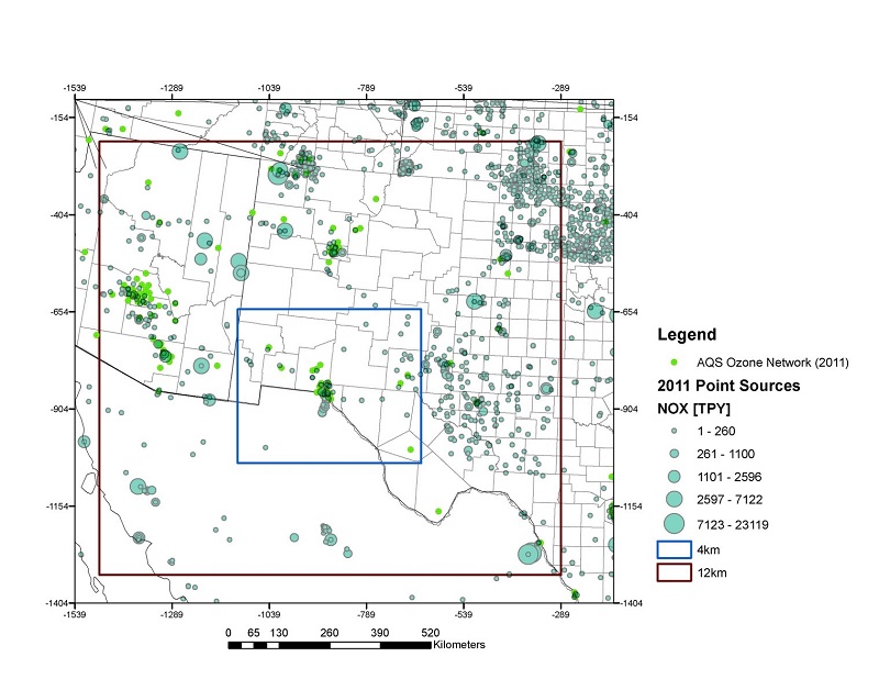
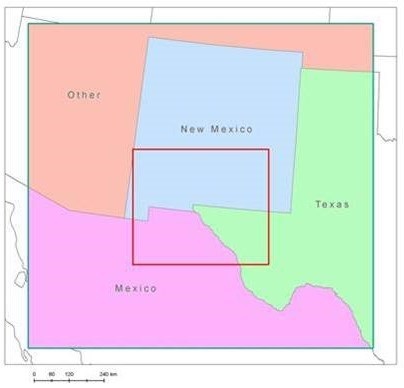
The SNMOS 2011 and 2025 ozone source apportionment simulations were conducted on the 12/4 km domain modeling shown in Figure 1 using Boundary Conditions (BCs) based on CAMx 2011 and 2025 regional model simulations of the continental U.S., respectively. Also shown in Figure 1 are the locations of the ozone monitors (green) and NOx point sources (blue) that include the Carbon coal-fired power plant located in Mexico in the southeast corner of the 12 km modeling domain and the Four Corners and San Juan coal-fired power plants in the northwest corner of New Mexico, as well as numerous compressors in the Permian Basin oil and gas development region just east of the 4 km modeling domain.
The CAMx OSAT ozone SA modelling tools provide separate hourly ozone contributions throughout the 12/4 km modeling domains for each user-selected Source Group. The source apportionment modeling provides a complete accounting of the contributions of all sources, so the Source Groups includes all emission sources. Source Groups are usually defined using a spatial map of geographic area Source Regions and providing as input different Source Categories of emission sectors, the intersection of a Source Region and Source Category defines a Source Group (e.g., on-road mobile source emissions from New Mexico). For the SNMOS CAMx 12/4 km ozone source apportionment simulations, four Source Regions (see Figure 2) and eight Source Categories were defined as follows:
Source Regions (4):
- New Mexico;
- Texas;
- Mexico; and
- Arizona and remainder of other states in the 12 km domain
Source Categories (8):
- Natural (biogenic and lightning NOx);
- On-Road Mobile;
- Non-Road Mobile;
- Oil and Gas (point and non-point);
- Electrical Generating Unit (EGU) Point;
- Non-EGU Point;
- Open Land Fires (wildfire, prescribed burns and agricultural burning); and
- Remainder Anthropogenic.
Initial concentrations (IC) and boundary conditions (BC) are always included as separate Source Groups resulting in a total of 34 Source Groups (34 = 4 x 8 + 2) for the SNMOS source apportionment modeling. Source apportionment simulations were performed with this same configuration for both the 2011 and 2025 emission scenarios.
SNMOS Source Apportionment Modeling Results
The ozone contributions of each Source Group to the current year (2011) and future year (2025) ozone Design Values and maximum daily 8-hour average (MDA8) ozone concentrations at each monitoring site within Doña Ana County and vicinity (i.e., the 4 km modeling domain) were analyzed several ways:
- Contributions of emissions from each Source Group, Source Region and Source Category to 2011 and 2025 ozone Design Values and MDA8 ozone concentrations.
- Section 179B analysis to assess the contributions of anthropogenic emissions from Mexico to ozone Design Values to demonstrate that “but for” emissions from Mexico Doña Ana County would have attained the October 2015 0.070 ppm ozone NAAQS.
- The source apportionment no Mexico 2011 ozone Design Values were compared to a CAMx no Mexico emissions zero-out sensitivity simulations and found similar contributions to ozone Design Values.
- Sensitivity of 2025 ozone Design Value projections without the influence of fires.
A summary of the SNMOS ozone source apportionment modeling results are available in the Task 12 SA Modeling PowerPoint Presentation with details on the ozone Design Value source apportionment modeling analysis available in an interactive Excel spreadsheet. To display the Source Group contributions to 2011 and 2025 MDA8 ozone concentrations, the modeling results were loaded into a web-based Source Apportionment Visualization Tool (SA Vis Tool) that are available for the 2011 and 2025 SA modeling results at:
SNMOS 2011 and 2025 SA Vis Tool
The SA Vis Tools generate pie charts of 2011 and 2025 ozone contributions by Source Region, Source Category or both (i.e., Source Groups) for monitoring sites within the SNMOS 4 km modeling domain. The application of the SA Vis Tool involves the following:
- Selection of whether ozone SA visualization is for the 2011 or 2025 emissions scenario.
- Selection of the monitor where data is requested. This request can be made either by selecting the monitor from drop down menus for State, County and Site or by using the map and selecting the monitor location.
- Select the day where results are desired. The day can be selected from a top five ozone day list, from a drop down menu of ranked ozone days from high to low during the May-Sep modeling period or from a calendar. Note that multiple days can also be selected and the SA Tool will visualize the average contribution across those days.
- The SA Vis Tool will then visualize the modeled 2011 or 2025 MDA8 ozone value for the selected monitoring site and day:
- The top bar in the plot will list the modeled 2011/2025 MDA8 ozone for the selected site/day(s), the amount the ozone is due to BCs around the 12/4 km SNMOS domain (Figures 1 and 2) and the amount of the rest of the ozone (Non-BC);
- For the 2011 SA Vis Tool the top bar will also list the observed MDA8 ozone on this site/day and the bias. The 2025 SA Vis Toll will leave the observed MDA8 ozone and bias locations blank.
- Initially, the upper pie chart will be the Non-BC ozone contributions by Source Regions;
- Initially, the lower pie chart will be the Non-BC ozone contributions by Source Categories;
- Next to the lower pie chart will be a 10-day time series centered on the day in question that shows total MDA8 ozone and ozone due to BC;
- The monitoring site or day can be changed using drop down menus in the top left corner of the Tool. The day can also be changed by clicking on the MDA8 ozone for a new day in the time series chart.
- The Region/Category pie charts can be switched.
- Clicking on one of the pie slices in the top pie chart provides more information in the bottom pie chart about that slice.
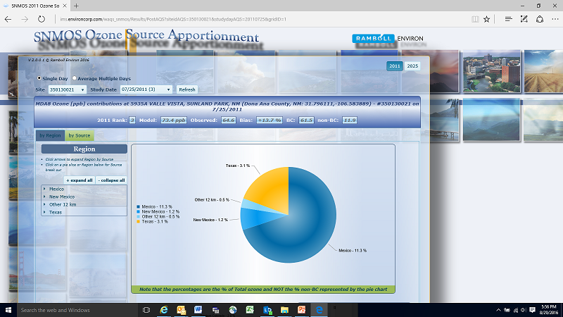
Figures 3, 4 and 5 displays an example from the SNMOS 2011 SA Vis Tool for the Desert View monitoring site in Doña Ana County, New Mexico (5935A Valle Vista, Sunland Park, NM #350130021) on July 25, 2011. The total modeled 2011 MDA8 ozone at Desert View on July 25, 2015 is 73.4 ppb, which is the third highest MDA8 ozone day at Desert View and is within 13.7% of the observed value (64.6 ppb). Of the 2011 modeled 73.4 ppb MDA8 ozone, 61.5 ppb (84%) is due to the BC and the remaining 11.9 ppb (16%) non-BC portion is due to emissions in the SNMOS 12/4 km modeling domain (Figures 1 and 2).
The pie charts show the ozone contributions from the non-BC portion of the MDA8 ozone (i.e., the 11.9 ppb component) with the percent numbers with the pie slices displaying the percent of total ozone (73.4 ppb). Initially, the upper pie chart displays ozone contributions by Source Regions (Figure 3) and the lower pie charts displays contributions by Source Categories (Figure 4). For Desert View on July 25, 2011, emissions from Mexico contribute 11.3% (8.3 ppb) of the total ozone (Figure 3) that is approximately 70% of the 11.9 ppb non-BC ozone contribution, with Texas and New Mexico contributing 3.1% (2.3 ppb) and 1.2% (0.9 ppb) to the total MDA8 ozone at Desert View on this day.
The lower pie chart displays contributions by Source Category that initially breaks down the total non-BC (11.9 ppb) contribution (Figure 4). The key to the definitions of the Local Source ozone SA modeling Source Contributions are as follows:
- NAT = Natural Emissions (Biogenic and Lightning NOx)
- FIRE = Wildfires, Prescribed Burns and Agricultural Burning
- MV = On-Road Mobile Source Emissions
- NR = Non-Road Mobile Source Emissions
- OG = Oil and Gas Emissions
- EGU = Electrical Generating Unit Point Source Emissions
- NEGU = Non-EGU Point Source Emissions
- OANT = Other Anthropogenic Emissions (Area Sources)
Of the 11.9 ppb ozone contributions within the 12/4 km modeling domain at Desert View on July 25, 2015, on-road mobile contributes the most (6.4% of total MDA8 ozone or 4.7 ppb), followed by Natural (3.2% or 2.4 ppb) and on-road mobile (2.7% or 2.0 ppb) (Figure 5). When a pie slice is selected in the top Source Region pie chart, the bottom Source Category pie chart displays the contributions of Source Categories to that Source Region. Figure 5 shows the Source Category pie chart for the Mexico slice from the Source Region pie chart (Figure 3). Note that the Mexico emissions inventory did not have as much information as the U.S. inventory to break down the emissions into the 8 Source Categories listed above. So for point sources we stratified the Mexico point sources into large emitters that were placed in the EGU Source Category if their NOx emission were over 5 tons per day (TPD) and lower emitters were put in the NEGU category. In addition, the Mexico inventory did not have separate codes for oil and gas sources (OG) so they are likely contained in the small point sources (NEGU) and other anthropogenic (OANT) Source Categories.