Winter Ozone AQ Modeling Results
Approach
The WAQS modeling team conducted a series of CAMx sensitivity simulations off of 3SAQS Base 2011 version A (CAMx_3SAQS04_B11a) with the objectives of understanding the deficiencies and improving the ability of the model in reproducing high wintertime ozone concentrations related to localized meteorological conditions and oil and gas emissions sources. The WRF Winter Modeling Workplan and WRF Winter Modeling Evaluation Report describe our efforts to improve the simulation of the meteorology associated with high wintertime ozone. The WRF modeling conducted by the WAQS team resulted in a wintertime WRF configuration that results in a better model of the inversion events that accompany high ozone concentrations.The WAQS modelers conducted a CAMx simulation with the new winter meteorology (and additional improvements to the way CAMx simulates snow albedo and chemistry). The changes to the meteorology did little to improve the CAMx under predictions of high wintertime ozone. Using insights from top down modeling and observational campaigns in Intermountain West oil and gas basins, the WAQS team developed a brute force oil and gas emissions sensitivity to test the hypothesis that our simulations underpredict VOC emissions and overpredict NOx emissions from oil and gas sources. The second winter O3 sensitivity used the same meteorology inputs as the winter meteorology simulation and included the following adjustments to the emissions from oil and gas sources (both area and point): 2x VOCs, 10x formaldehyde, and 0.5x NOx. While the emissions perturbation produced improvements at some monitoring locations at some times, there were still high ozone events that were badly underpredicted by the model.
The final CAMx sensitivity simulation conducted by the WAQS modelers was designed to test the hypothesis that there was still to much dilution in the surface layer of the model. The winter ozone layer sensitivity used the adjusted oil and gas emissions and the WRF winter meteorology. The WAQS modelers adjusted the WRFCAMx processor to use the same vertical layer structure as WRF within the first 6 model layers. In all of the previous simulations (base, winter met, oil and gas emissions) the first 6 WRF layers were collapsed into the 3 CAMx layers such that WRF layers 1+2 = CAMx layer 1, WRF layers 3+4 = CAMx layer 2, and WRF layers 5+6 = CAMx layer 3. This collapsing roughly amounted to 12 m deep WRF layers being collapsed to 24 m deep CAMx layers. In the vertical mixing sensitivity the WRF vertical layer structure was preserved for the first 6 layers resulting in 28 layer CAMx meteorology (compared to 25 layer meteorology in the previous runs). Note that there was still layer collapsing applied above the first 6 WRF layers.
Simulation Summary:
Base Simulation (Base11a)
Simulation ID: CAMx_3SAQS04_B11a
Modeling Period: February 1-March 31, 2011
Analysis Domain: 4-km
Meteorology Sensitivity (WinterO3)
Simulation ID: CAMx_3SAQS04_B11a_WinterO3
Met: WRF Winter + WRFCAMx Snow 25 layers
Emissions: Same as CAMx_3SAQS04_B11a
Oil and Gas Emissions Sensitivity (OG_Emis)
Simulation ID: CAMx_3SAQS04_B11a_WinterO3_OG_Emis
Met: Same as CAMx_3SAQS04_B11a_WinterO3
Emissions: 2x O&G VOC, 10x O&G HCHO, 0.5x O&G NOx adjustments to CAMx_3SAQS04_B11a
Vertical Transport Sensitivity (Layers)
Simulation ID: CAMx_3SAQS04_B11a_WinterO3_OG_Emis_Layers
Met: WRF Winter + WRFCAMx Snow 28 layers (no collapsing in layers 1-6)
Emissions: Same as CAMx_3SAQS04_B11a_WinterO3_OG_Emis
Results
The results of the winter O3 modeling simulations are shown first as high level summaries of the domain wide performance and then as site-level performance plots.Performance Tables
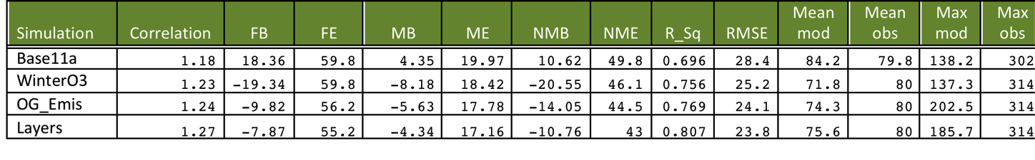
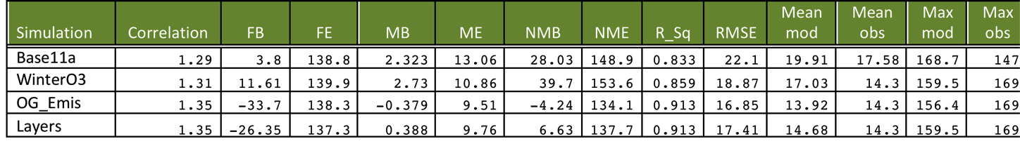
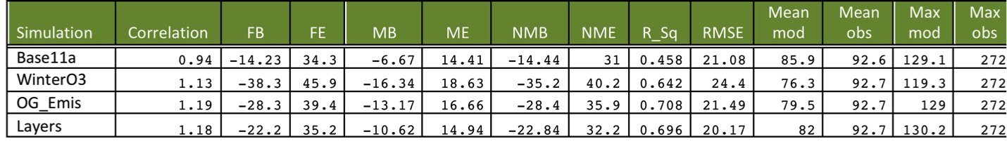
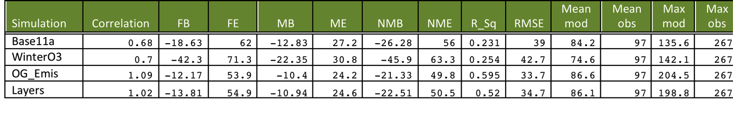
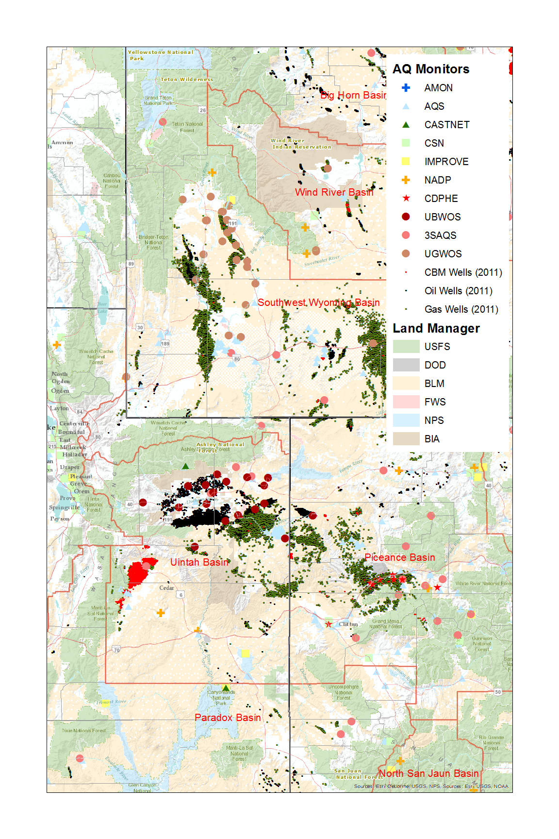
The tables below present performance statistics averaged across all sites and all days for the months of February and March 2011. The header for each table lists the applicable monitoring network and pollutant. The networks presented here all include oil and gas development areas, although some of the networks (UGWOS and Uintah Basin) are more selective of only oil and gas development locations than others (AQS).
AQS Hourly O3 sites in the 4-km Domain
AQS Hourly NO2 sites in the 4-km Domain
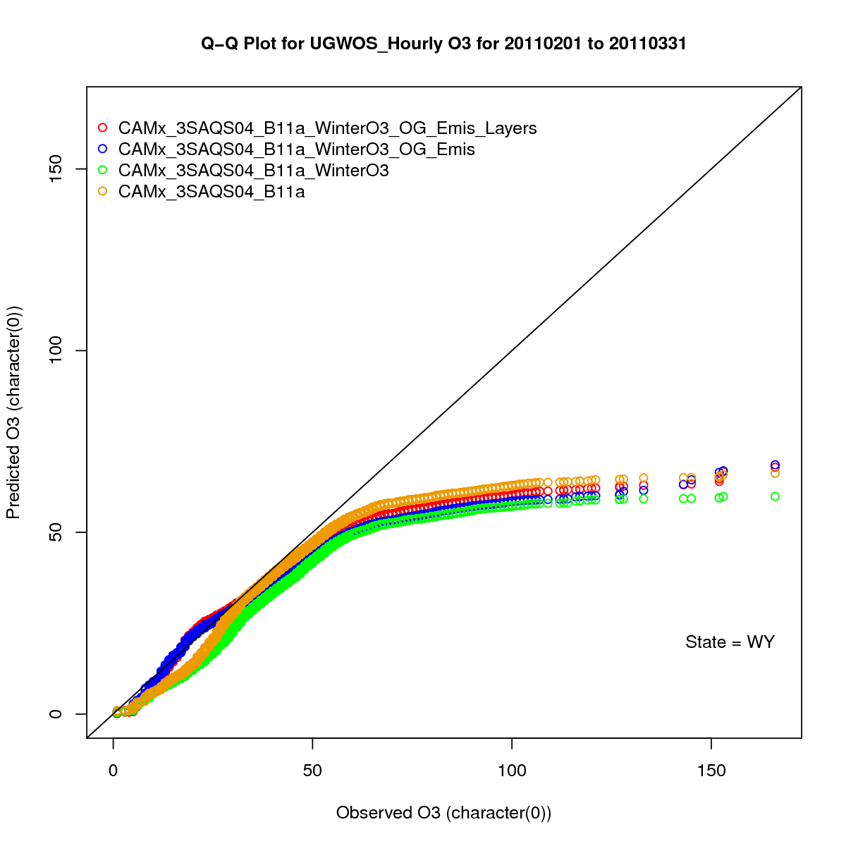
Upper Green River Basin, WY Hourly O3 sites
Upper Green River Basin, WY Hourly NO2 sites

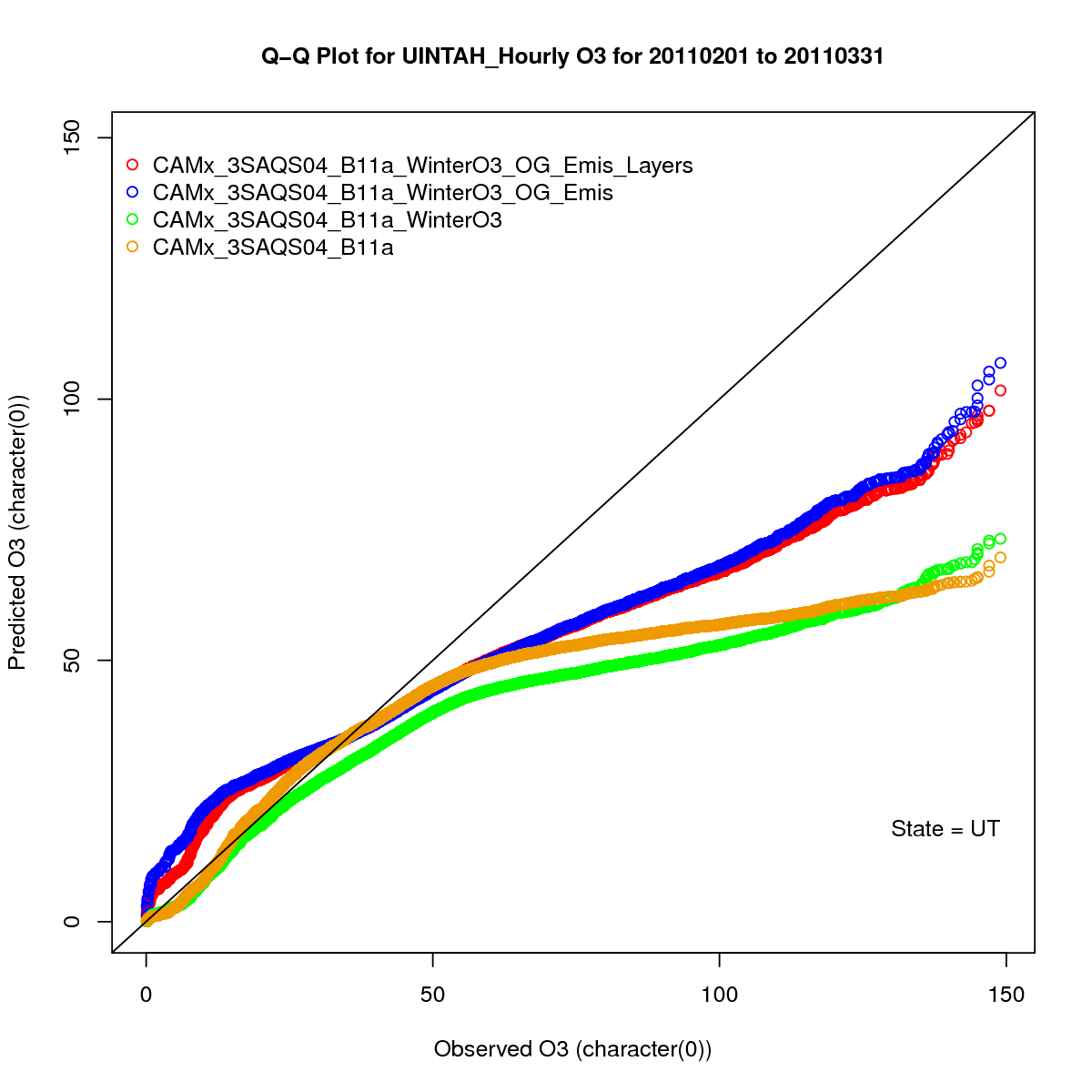
Uintah Basin, UT Hourly O3 sites
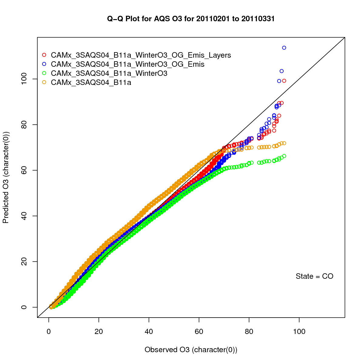
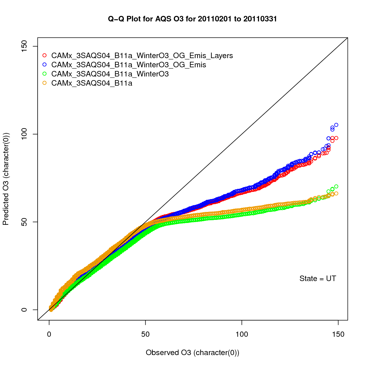
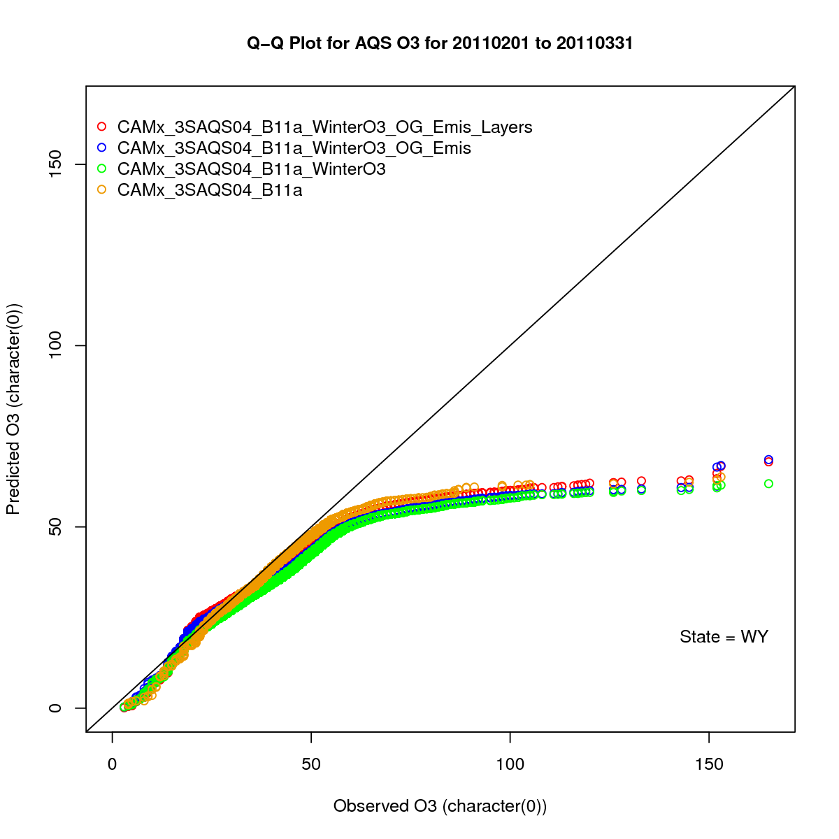
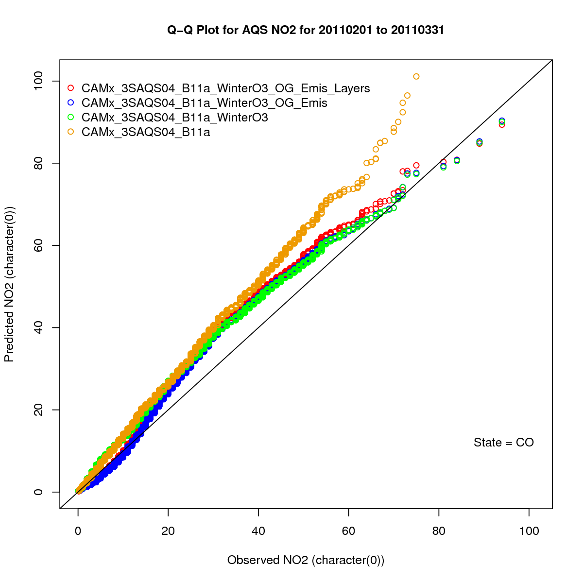
Q-Q Plots
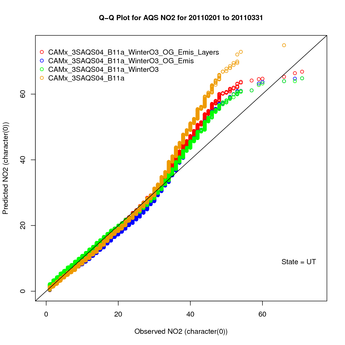
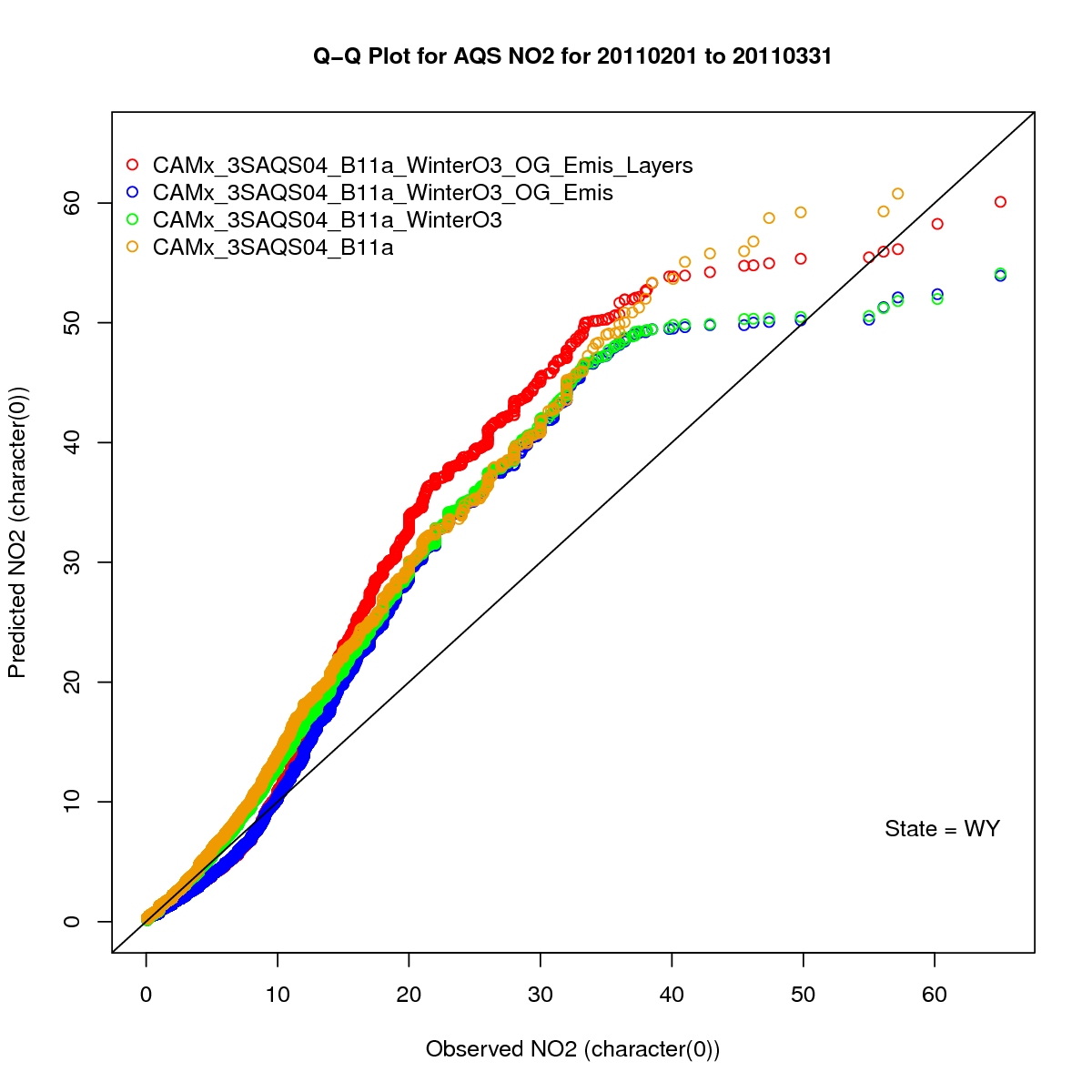
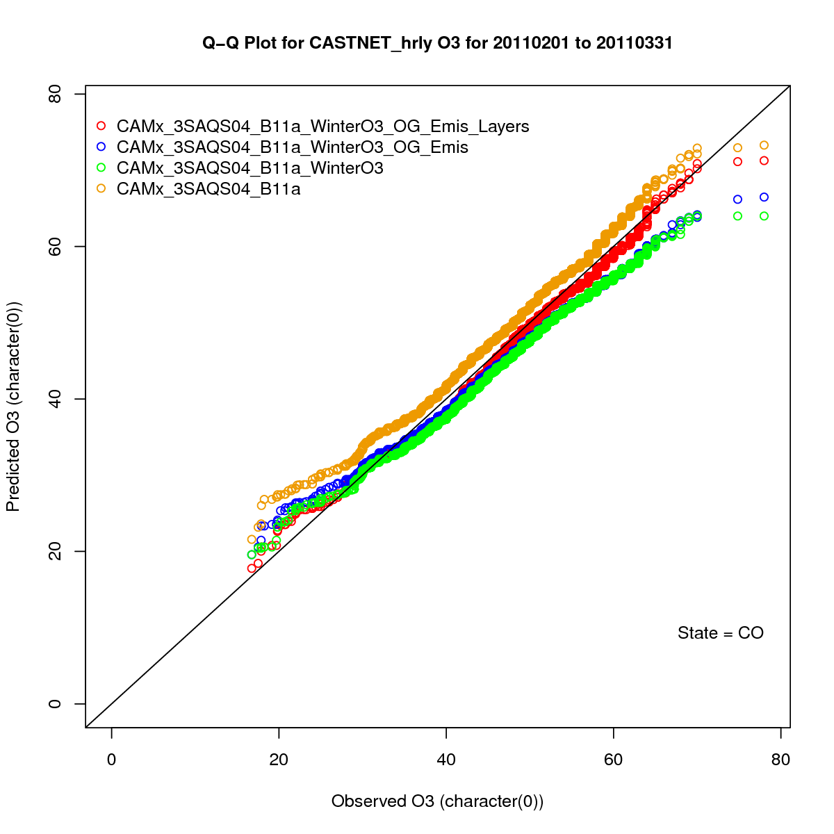
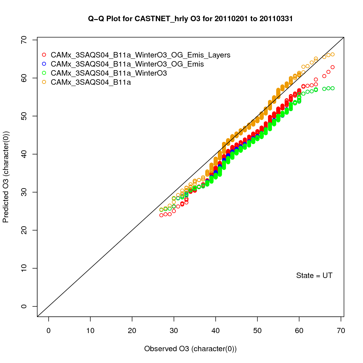
In traditional Quantile-Quantile (Q-Q) plots two probability distributions are plotted against each other. This concept is modified here for air quality data by plotting two concentration distribution against (model vs obs) each other. In the Q-Q plots below all of the observations and model results for a given time period and set of locations are matched and then unpaired and sorted from low to high concentrations. These plots highlight the skill of the model at simulating the range of observed concentrations.
Hourly O3 at AQS Sites: February-March 2011 (units=ppb)
| Colorado AQS | Utah AQS | Wyoming AQS |
|---|---|---|
 |  |  |
| Colorado AQS | Utah AQS | Wyoming AQS |
|---|---|---|
 |  |  |
| Colorado CASTNet | Utah CASTNet | Wyoming CASTNet |
|---|---|---|
 |  | 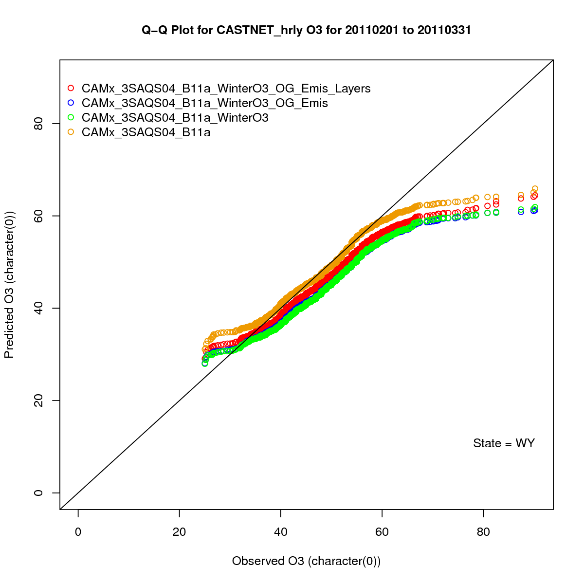 |
 |
 |
Timeseries Analysis
The time series plots here compare hourly observed and modeled O3 and NO2 at the AQS (CO,UT,WY), Uintah Basin (UT), and Upper Green River Basin (WY) monitoring sites. The dual-pane plots shows the hourly concentrations on the top pane and hourly bias on the bottom pane. Time series plots of O3, NO2, and VOCs (where available) for individual sites in Colorado, Utah, and Wyoming are available on the IWDW.Hourly O3 at AQS Sites: February-March 2011 (units=ppb)
| Colorado AQS | Utah AQS | Wyoming AQS |
|---|---|---|
 |  |  |
| Colorado AQS | Utah AQS | Wyoming AQS |
|---|---|---|
 |  |  |
 |
| O3 | NO2 |
|---|---|
 |  |
Discussion
The emissions and layer collapsing sensitivity simulations generally improved the average modeled O3 and NO2 performance at the AQS and Uintah Basin monitoring networks. The correlation coefficient and R^2 increased while the bias and error metrics decreased in these simulations relative to the base case. The winter O3 configuration produced worse average performance (higher NMB and NME than the base) in most of the networks.
The Q-Q plots highlight the response of the model in simulating air quality at the different monitoring networks to the sensitivities. At the upper end of the observed concentration range, the simulated O3 at the AQS sites in CO and UT responded favorably to the emissions and layer sensitivities; the O3 concentrations at the WY AQS sites did not show as drastic a change as the other states. The NO2 concentrations at the AQS sites in all three states were more responsive to the meteorology changes than either the chemistry or layers sensitivities. The Q-Q plot for Uintah hourly ozone demonstrates that the model is most improved by the emissions sensitivity, which is consistent with the fact that the emissions perturbations (2x VOC, 10x HCHO, and 0.5x NOx) were derived from a top down analysis of sites in the Unitah Basin. The O3 model for the Upper Green River Basin sites did not respond favorably to any of the sensitivity configurations, particularly the meteorology changes.
The time series analyses confirm the conclusion that the winter O3 configurations improved the model performance at the sites in Eastern Utah and Northwest Colorado (Uintah), while the model either stayed the same or degraded for sites in Southwest Wyoming (Upper Green) and Western Colorado (Piceance). Promising improvements in O3 performance at some sites in Utah (e.g. Horsepool and Ouray) indicate that while the meteorology and emissions changes moved the model in the right direction there are still deficiencies in the representation of the dynamical and chemical conditions producing high wintertime O3.
The changes in model performance at the Upper Green River Basin sites indicate that the model is likely missing important dynamical features that lead to high ozone concentrations. At sites that experience episodic high O3, the model performs fairly well in simulating the typical daytime O3 concentrations (e.g. Daniel). This trend indicates that the emissions magnitudes are well represented at these locations. The model is missing the development of strong temperature inversions, atypical emissions events (i.e. completions and blowdowns), or both, that lead to high ozone. The slight improvement in model performance during high ozone periods resulting from the layer sensitivity illustrates that the shallower surface layer in this configuration is a step in the right direction. A clue to whether the high ozone is from atypical emission increases or dynamics (i.e. inversions) may be seen in the Upper Green River Basin network wide timeseries plot. This plot shows high average ozone across all sites in the network, which would indicate a meteorological driver rather than emissions, as the impacts of localized emissions increases should only be seen at monitors nearby the sources with atypical operations.
Increasing the VOC emissions at the Piceance Basin sites was not favorable to VOC model performance (e.g. Rifle total VOCs).
The sensitivity modeling results show that domain-wide configuration changes are not sufficient to improve the model performance at the most important locations: the monitoring sites measuring non-attainment for O3. Although the domain-wide performance improved with the sensitivities, the sensitivity configurations did not have the precision to target the model performance issues at individual sites. In general, the meteorology and emissions sensitivities produced the best results at the Uintah Basin sites. This result makes sense because the meteorology changes to improve the simulation of cold pools and the emissions changes were both derived from studies of the Uintah Basin. Despite these improvements, problems still exist in the Uintah Basin O3 model, particularly in capturing the magnitude and persistence of high O3. None of the sensitivity configurations were particularly effective at improving the O3 model performance in the Upper Green or Piceance Basins.
Recommendations for Future Work
Additional Materials
Emissions Adjustments Notes
Published O&G Basin Emission Adjustment Factors
| Basin | NOx | VOC | CH4 | Notes | Reference |
|---|---|---|---|---|---|
| Denver-Julesberg | >2.0 | Petron et al., 2012 | |||
| Piceance | |||||
| North San Juan | |||||
| South San Juan | |||||
| Paradox | |||||
| Uintah | 0.25 | 1.6 | 4.4 | Uintah and Duchesne Counties | Karion et al., 2013; Ahmadov et al., 2015 |
| Southwest Wyoming | |||||
| Big Horn | |||||
| Wind River | |||||
| Powder River | |||||
| Great Plains | |||||
| Williston |
Upper Green River Basin CAMx Analysis
Monthly Average Concentrations
| Big Piney | VOC | CH4 | |||||
| Boulder | VOC | CH4 | Winter VOC | Winter CH4 | Winter NO2 | Hourly CH4 | Hourly NO2 |
| Gillette | VOC | CH4 | |||||
| Pavilion | VOC | CH4 | Winter VOC | Winter CH4 | Winter NO2 | ||
| Wamsutter | VOC | CH4 |
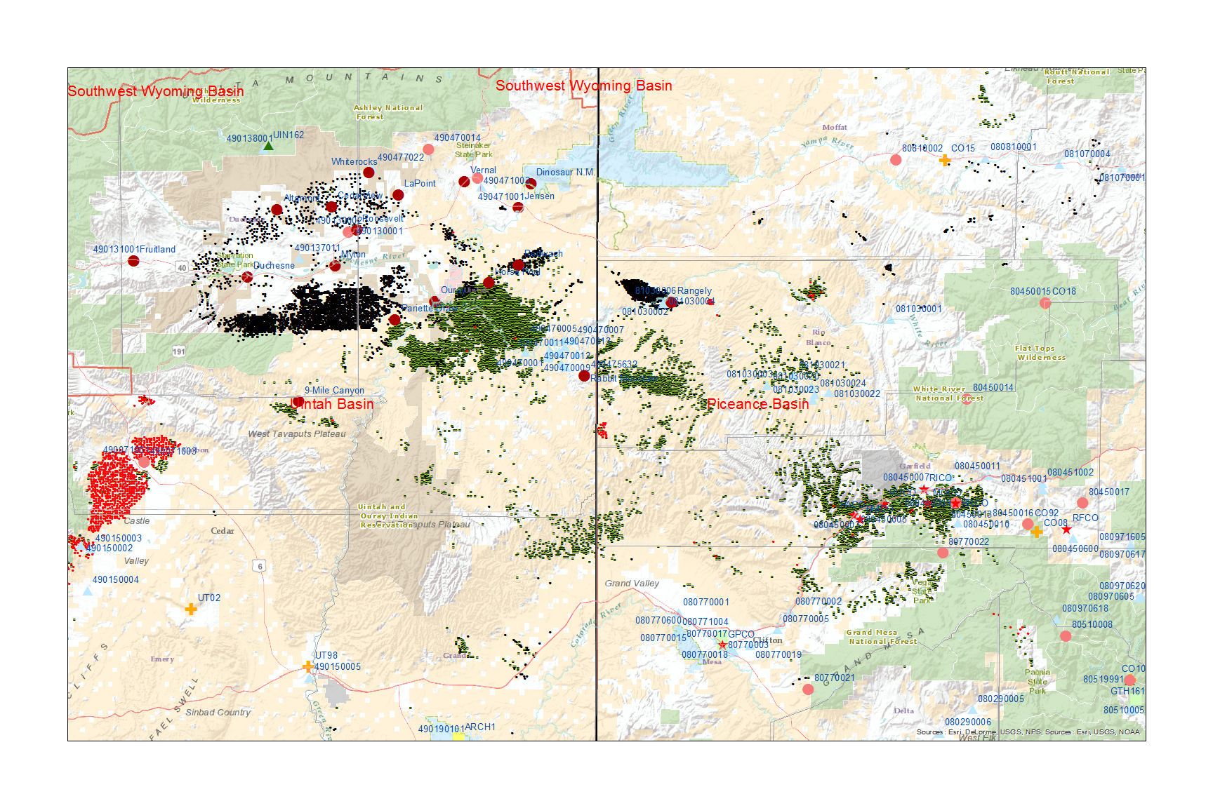
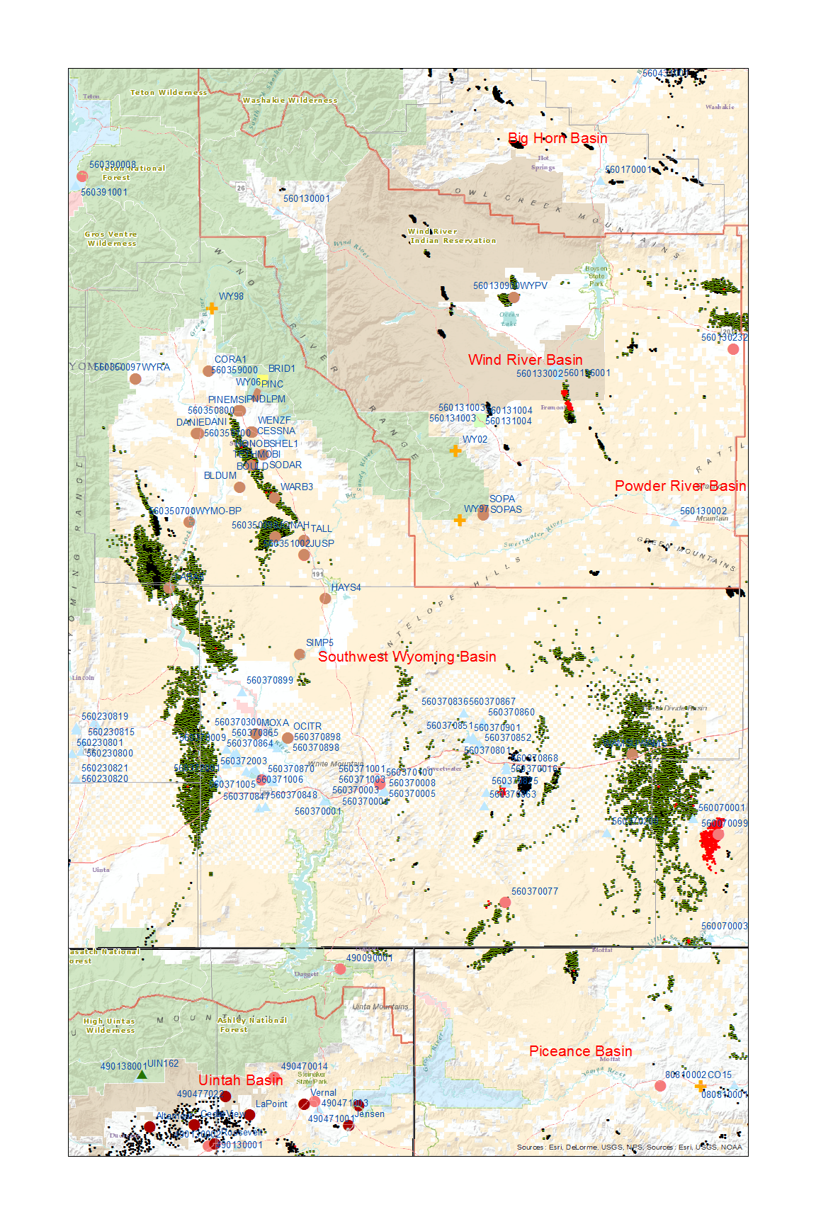
Monitoring Maps
Etc.
Uintah Basin Winter Ozone Study
These sites only measured ozone and meteorology parameters
| Site | Lat, Long, Elev | Time-Height | ||
|---|---|---|---|---|
| Altamount | 40.3603, -110.2858, 1949.8056 | Feb, Mar | ||
| Cedarview | 40.383524, -110.072563, 1692.2496 | |||
| Feb 12-16 | >135 ppb | WRF-Winter | ||
| Feb 23-24 | >100 ppb | |||
| Mar 1-3 | >90 ppb | WRF-Winter | ||
| Dinosaur | 40.4371, -109.3047, 1462.7352 | Jan 6-9 | >80 ppb | |
| Feb 12-16 | >110 ppb | WRF-Winter | ||
| Duchesne | 40.1615, -110.4011, 1682.496 | Jan 29-30 | >90 ppb | |
| Feb 12-16 | >120 ppb | WRF-Winter | ||
| Horse Pool | 40.1437, -109.4672, 1569.4152 | Jan 6-8 | >100 ppb | |
| Jan 24-31 | >95 ppb | |||
| Feb 12-16 | >130 ppb | WRF-Winter | ||
| Feb 23-25 | >120 ppb | |||
| Mar 1-4 | >115 ppb | WRF-Winter | ||
| Jensen | 40.3671, -109.3522, 1450.848 | Feb 12-16 | >100 ppb | WRF-Winter |
| Feb 23-24 | >80 ppb | |||
| Mar 1-2 | >80 ppb | WRF-Winter | ||
| Lapoint | 40.404, -109.8157, 1673.9616 | Jan 6-8 | >90 ppb | |
| Jan 27-31 | >80 ppb | |||
| Feb 12-16 | >120 ppb | |||
| Feb 22-24 | >100 ppb | |||
| Mar 1-3 | >85 ppb | |||
| Ouray | 40.054768, -109.688001, 1463.9544 | Jan 6-9 | >100 ppb | |
| Jan 16-17 | >95 ppb | |||
| Jan 26-31 | >105 ppb | |||
| Feb 11-16 | >140 ppb | |||
| Feb 24-25 | >120 ppb | |||
| Mar 1-3 | >100 ppb | |||
| Pariette Draw | 40.03460278, -109.8300556, 1466.6976 | Feb 11-16 | >140 ppb | |
| Feb 22-25 | >120 ppb | |||
| Mar 1-3 | >110 ppb | |||
| Rabbit Mountain | 39.8687, -109.0973, 1878.7872 | Jan 16 | >85 ppb | |
| Feb 14-16 | >100 ppb | |||
| Red Wash | 40.1972, -109.3525, 1688.8968 | Jan 6-9 | >95 ppb | |
| Jan 26-31 | >95 ppb | |||
| Feb 12-15 | >135 ppb | |||
| Feb 23-24 | >105 ppb | |||
| Mar 1-3 | >100 ppb | |||
| Roosevelt | 40.30073056, -109.9784172, 1544.7264 | Jan 6-9 | >80 ppb | |
| Jan 27-31 | >100 ppb | |||
| Feb 12-16 | >120 ppb | WRF-Winter | ||
| Feb 3-4 | >100 ppb | |||
| Mar 1-3 | >80 ppb | |||
| Vernal | 40.443273, -109.560983, 1662.684 | Jan 8-9 | >85 ppb | |
| Feb 12-16 | >100 ppb | WRF-Winter | ||
| Feb 24 | >85 ppb | |||
| Mar 2 | >80 ppb |
| Site | Lat, Long, Elev | 2011 Episode Dates | 8-hr O3 Concentrations | Obs Y/N |
|---|---|---|---|---|
| Wyoming Range | 42.98, -110.35, 2475 | Feb 15 | >80 ppb | Y |
| Mar 10 | >80 ppb | |||
| Pinedale | 42.92, -109.79, 2388 | Mar 1-2 | >85 ppb | Y |
| Mar 5 | >80 ppb | |||
| Juel Springs | 42.37, -109.56, 2144 | Mar 2 | >90 ppb | Y |
| Mar 12 | >85 ppb | |||
| Mar 15 | >85 ppb | |||
| Daniel | 42.79, -110.05, 2173 | Mar 10 | >80 ppb | Y |
| Boulder | 42.71, -109.75, 2160 | Feb 14 | >85 ppb | Y |
| Mar 1-5 | >120 ppb | |||
| Mar 12 | >120 ppb | |||
| Mobile Trailer | 42.68, -109.8, 2143 | Feb 14 | >80 ppb | Y |
| Mar 3 | >80 ppb |